Tugas Besar Metode Numerik - Josiah Enrico S
Contents
Abstract
Introduction
Objective
- Membuat program analisis truss dan optimasi sederhana dengan Modelica
- Mengoptimasi harga pembuatan rangka truss sederhana dengan memvariasi dimensi dan elastisitas material.
Methodology
- Metode Optimasi Golden Section (univariabel)
- Metode Optimasi Golden Section (multivariabel)
Procedure
Geometri dan Load
| F1 | 2000 |
|---|---|
| F2 | 1000 |
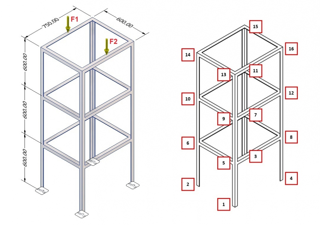
Figure 1 Truss geometry and load

Constraint:
- Spesifikasi L (Panjang) dan geometri rangka truss
- Gaya beban terhadap struktur (1000 N dan 2000 N)
Asumsi:
- Beban akan terdistribusi hanya pada point penghubung dan semua gaya yang dipengaruhi moment diamggap tidak ada karena sistem bersifat truss
Koleksi Data
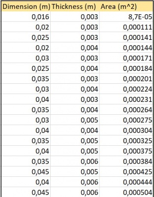
Table 1 Angle bar standard dimension and area
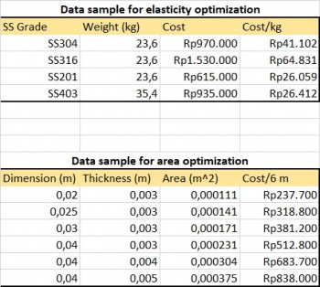
Table 2 Cost of material in market


Data Proceessing
Truss Structure Analysis Model
Pada tahap pertama, dilakukanka simulasi menggunakan Modelica untuk mengetahui pengaruh beban gaya yang diberikan terhadap struktur truss. Pengaruh ini direpresantasikan oleh 4 nilai yaitu displacement/perpindahan, gaya reaksi, tekanan di setiap truss dan faktor keamanan di setiap truss. Keempat nilai ini diperoleh dengan menggunakan operasi tranformasi matriks untuk pembebanan truss dalam Finite Element Analysis. Operasi ini diterjemahkan ke dalam bahasa C dalam pemrograman Modelica. Berikut ini adalah hasil simulasi Modelica dan program tertulisnya:

Figure 2 Modelica Simulation Result of point displacement, reaction force, each truss stress, each truss safety factor

model Truss_3D_Tugas_Besar_Safety
// Base Code by Josiah Enrico S. 1906356286
// Editing and Testing by Ahmad M. Fahmi 1806181836
// Commenting and Cleaning by Christopher S. Erwin 1806201056

// === DEFINITION PHASE ===

// Define the properties of the truss arrangement
parameter Integer Nodes = size(node_points,1);    // Number of Nodes
parameter Integer Members = size(node_pairs,1);   // Number of Members

// Define the properties of the truss material
parameter Real Yield = 215e6;           // Yield Strength (Pa)
parameter Real Area = 0.000224;         // Area L Profile [Dimension=0.03, Thickness=0,004] (m^2)
parameter Real Elas = 193e9;            // Elasticity of material [SS 304] (Pa)

// Define connections; list pair of nodes joined by a member
parameter Integer node_pairs[:,2]=[1,5; 2,6; 3,7; 4,8;         // Lowest vertical members
                                  5,6; 6,7; 7,8; 5,8;         // 1st shelf
                                  5,9; 6,10; 7,11; 8,12;      // Middle vertical members
                                  9,10; 10,11; 11,12; 9,12;   // 2nd shelf
                                  9,13; 10,14; 11,15; 12,16;  // Top vertical members
                                  13,14; 14,15; 15,16; 13,16];// 3rd shelf

// Define coordinates and boundaries of each node
// [x, y, z, boundary_x, boundary_y, boundary_z]
// If the node is bound (stationary) along that axis, then boundary_axis = 1
// otherwise the node is free and boundary_axis = 0
parameter Real node_points[:,6]=[0.3,-0.375,0,1,1,1;      // Node 1
                                -0.3,-0.375,0,1,1,1;     // Node 2
                                -0.3,0.375,0,1,1,1;      // Node 3
                                0.3,0.375,0,1,1,1;       // Node 4

                                0.3,-0.375,0.6,0,0,0;    // Node 5
                                -0.3,-0.375,0.6,0,0,0;   // Node 6
                                -0.3,0.375,0.6,0,0,0;    // Node 7
                                0.3,0.375,0.6,0,0,0;     // Node 8

                                0.3,-0.375,1.2,0,0,0;    // Node 9
                                -0.3,-0.375,1.2,0,0,0;   // Node 10
                                -0.3,0.375,1.2,0,0,0;    // Node 11
                                0.3,0.375,1.2,0,0,0;     // Node 12

                                0.3,-0.375,1.8,0,0,0;    // Node 13
                                -0.3,-0.375,1.8,0,0,0;   // Node 14
                                -0.3,0.375,1.8,0,0,0;    // Node 15
                                0.3,0.375,1.8,0,0,0];    // Node 16

// Define external forces in Newtons on each node
// [Fx, Fy, Fz]
parameter Real Forces[nodes_xyz]={0,0,0,      // Node 1
                                 0,0,0,      // Node 2
                                 0,0,0,      // Node 3
                                 0,0,0,      // Node 4
                                 0,0,0,      // Node 5
                                 0,0,0,      // Node 6
                                 0,0,0,      // Node 7
                                 0,0,0,      // Node 8
                                 0,0,0,      // Node 9
                                 0,0,0,      // Node 10
                                 0,0,0,      // Node 11
                                 0,0,0,      // Node 12
                                 0,0,-500,   // Node 13
                                 0,0,-1000,  // Node 14
                                 0,0,-1000,  // Node 15
                                 0,0,-500};  // Node 16

// === SOLUTION PHASE ===

Real displacement[nodes_xyz], reaction[nodes_xyz];
Real check[3]; // To check if forces in xyz directions sum to zero (structure is static)

Real safety[Members];     // Safety Factor of each member (based on stress experienced)
Real mem_dis[3];          // Displacement in xyz directions experienced by member
Real stress_vector[3];    // Stress experienced by member in xyz directions
Real stress_mag[Members]; // Magnitude of stress experienced by member

protected
parameter Integer nodes_xyz = 3 * Nodes;  // Size of vector of {node_#_x, node_#_y, node_#_z} containing all nodes
Real node_i[3], node_j[3];                // Coordinates in xyz for member's node pairs

// Global Stiffness Matrix construction
Real G_element[nodes_xyz, nodes_xyz], G_total[nodes_xyz, nodes_xyz], G_total_new[nodes_xyz, nodes_xyz];

// Transformation Matrix construction
Real cos_x, cos_y, cos_z, L, T[3,3];

// Limits to eliminate Float Errors
Real err_solve = 10e-10, err_check = 10e-4;

algorithm
//Creating Global Matrix
G_total := identity(nodes_xyz);

for mem in 1:Members loop
 // Get coordinates of member's nodes
 for i in 1:3 loop
   node_i[i] := node_points[node_pairs[mem,1],i];
   node_j[i] := node_points[node_pairs[mem,2],i];
 end for;

 // Finding the Stiffness Matrix [Ke]
 // {F} = [Ke]{U}
 // [Ke] = k[T]
 L := Modelica.Math.Vectors.length(node_j - node_i);
 cos_x := (node_j[1]-node_i[1])/L;
 cos_y := (node_j[2]-node_i[2])/L;
 cos_z := (node_j[3]-node_i[3])/L;
 T := (Area * Elas / L)*[cos_x^2,cos_x*cos_y,cos_x*cos_z;
                         cos_y*cos_x,cos_y^2,cos_y*cos_z;
                         cos_z*cos_x,cos_z*cos_y,cos_z^2];

 // Transforming to Global Matrix
 G_element := zeros(nodes_xyz,nodes_xyz);
 for m,n in 1:3 loop
   G_element[3*(node_pairs[mem,1]-1)+m, 3*(node_pairs[mem,1]-1)+n] :=  T[m,n];
   G_element[3*(node_pairs[mem,2]-1)+m, 3*(node_pairs[mem,2]-1)+n] :=  T[m,n];
   G_element[3*(node_pairs[mem,2]-1)+m, 3*(node_pairs[mem,1]-1)+n] := -T[m,n];
   G_element[3*(node_pairs[mem,1]-1)+m, 3*(node_pairs[mem,2]-1)+n] := -T[m,n];
 end for;

 // Adding to total Global Matrix
 G_total_new := G_total + G_element;
 G_total := G_total_new;
end for;

//Implementing boundary conditions to Global Matrix
for nod in 1:Nodes loop
 // Boundary x-axis
 if node_points[nod,4] <> 0 then
   for i in 1:Nodes*3 loop
     G_total[(nod*3)-2,i] := 0;
     G_total[(nod*3)-2,(nod*3)-2] := 1;
   end for;
 end if;

 // Boundary y-axis
 if node_points[nod,5] <> 0 then
   for i in 1:Nodes*3 loop
     G_total[(nod*3)-1,i] := 0;
     G_total[(nod*3)-1,(nod*3)-1] := 1;
   end for;
 end if;

 // Boundary z-axis
 if node_points[nod,6] <> 0 then
   for i in 1:Nodes*3 loop
     G_total[nod*3,i] := 0;
     G_total[nod*3,nod*3] := 1;
   end for;
 end if;
end for;

// Solving displacement (U)
// [G_total]{U} = {F}
displacement := Modelica.Math.Matrices.solve(G_total, Forces);

// Solving reaction (R)
// {R} = [G_total]{U} - {F}
reaction := (G_total_new * displacement) - Forces;

// Eliminating float errors
for i in 1:nodes_xyz loop
reaction[i] := if abs(reaction[i])<= err_solve then 0 else reaction[i];
displacement[i] := if abs(displacement[i])<= err_solve then 0 else displacement[i];
end for;

// Checking Sum of Forces
// For static structures, should add up to 0
check[1]:=sum({reaction[i] for i in (1:3:(nodes_xyz-2))}) + sum({Forces[i] for i in (1:3:(nodes_xyz-2))});
check[2]:=sum({reaction[i] for i in (2:3:(nodes_xyz-1))}) + sum({Forces[i] for i in (2:3:(nodes_xyz-1))});
check[3]:=sum({reaction[i] for i in (3:3:(nodes_xyz))}) + sum({Forces[i] for i in (3:3:(nodes_xyz))});

// Eliminating float errors
for i in 1:3 loop
 check[i] := if abs(check[i])<= err_check then 0 else check[i];
end for;

// === POSTPROCESSING PHASE ===

//Calculating stress in each truss
for mem in 1:Members loop
 // Getting node coordinate data and displacement for current member
 for i in 1:3 loop
   node_i[i] := node_points[node_pairs[mem,1],i];
   node_j[i] := node_points[node_pairs[mem,2],i];
   mem_dis[i] := abs(displacement[3*(node_pairs[mem,1]-1)+i] - displacement[3*(node_pairs[mem,2]-1)+i]);
 end for;

 // Solving the Displacement Matrix for current member
 // Stress = F/A = (E/L) * [dL]
 L:=Modelica.Math.Vectors.length(node_j-node_i);
 cos_x:=(node_j[1]- node_i[1])/L;
 cos_y:=(node_j[2]- node_i[2])/L;
 cos_z:=(node_j[3]- node_i[3])/L;
 T := (Elas/L)*[cos_x^2,cos_x*cos_y,cos_x*cos_z;
               cos_y*cos_x,cos_y^2,cos_y*cos_z;
               cos_z*cos_x,cos_z*cos_y,cos_z^2];

 stress_vector:=(T*mem_dis); // The stress in vector components {stress_x, stress_y, stress_z}
 stress_mag[mem]:=Modelica.Math.Vectors.length(stress_vector); // Magnitude/length of the stress vectors for each member
end for;

// Safety Factor
// Factor of Safety = (Yield Strength of material) / (Stress experienced by Member)
for mem in 1:Members loop
 if stress_mag[mem]>0 then
   safety[mem] := Yield / stress_mag[mem];
 else
   safety[mem] := 0;
 end if;
end for;

end Truss_3D_Tugas_Besar_Safety;
|
Cost and Cost Efficiency of Area Variation and Constrained Elasticity
Berdasarkan hasil analisis dari struktur truss sebelumnya, pada bagian ini parameter area cross-section dari setiap truss dalam struktur tesebut divariasi dengan menggunakan yann standar ukuran yang tertera pada prosedur. Data perbedaan Area dalam material yang sama tersebut diproses menjadi variasi harga (cost) dan efisiensi harga (safaty factor/cost) agar dapat diproses di akhir dengan optimisasi metode Powell. Dalam Prosesnya, data harga material yang terbatas di pasar akan di-regresi orde 2 untuk mendapatkan nilai harga pada ukuran-ukuran yang tidak memilik harga. Berikut adalah tabel hasil proses data dan grafik yang dihasilkan:
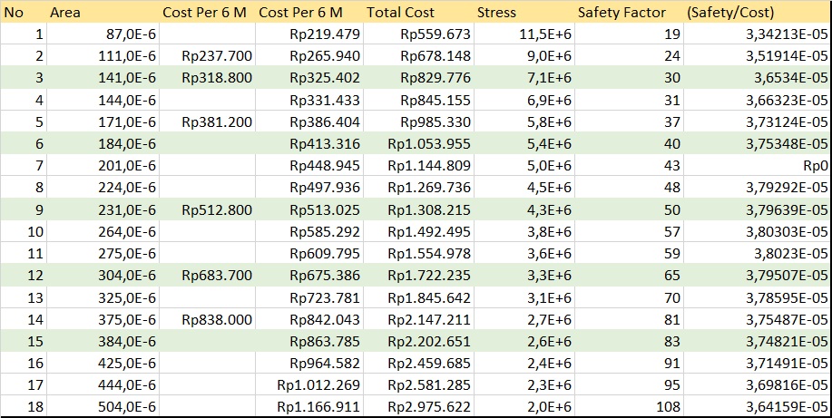
Table 3 Table of cost and cost efficiency

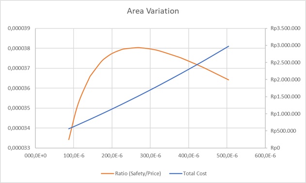
Figure 3 Graph of cost and cost efficiency

Cost and Cost Efficiency of Elasticity Variation and Constrained Area
Mirip dengan pengolahan data sebelumnya, bagian ini juga akan menghasilkan nilai variasi harga (cost) dan efisiensi harga (safaty factor/cost) untuk diolah dengan optimisasi metode powell di akhir. Namun, berbeda dengan sebalumnya, pada bagian ini area cross section akan disamakan nilainya dan elastisitas material akan divariasikan. Dalam pengolah ini, metode curve fitting orde 2 juga dilakukan untuk mendapatkan nilai-nilai harga, kekuatan yield, densitas yang kosong. Berikut adalah tabel hasil proses data dan grafik yang dihasilkan:
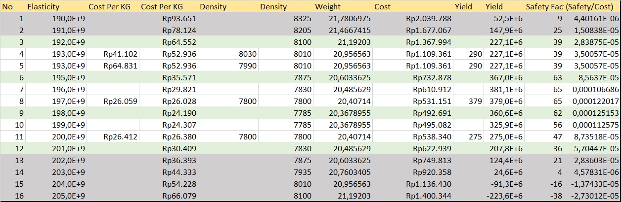
Table 4 Table of cost and cost efficiency

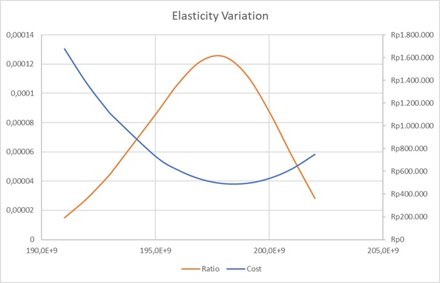
Figure 4 Graph of cost and cost efficiency

Result and Analysis
Hasil dari studi ini adalah nilai cost efficincy optimal yang dipengaruhi oleh 2 faktor yaitu elastisitas dan area. Oleh karena itu jenis optimisasi yang dilakukakn adalah optimasi multivariabel (lebih dari satu variabel) dengan metode powell. Metode ini dipilih karena tergolong cukup sederhana dan cepat mencapai titik konvergen. Secara singkat, agar lebih memahami optimasi multivariabel ini, bisa dibayangkan distribusi cost efficieny digambarkan sebagi grafik 3 dimensi dalam sumbu x, y, z, Cost efficiency akan diwakili skala z, elastisitas sebagai skala y dan area sebagai skala x. Nilai dari cost efficincy(z) pada suatu titik adalah fungsi area(x) dan elastisitas (y). Persamaan kuadrat cost efficiency yang diperolah dari curve fitting tahap sebelumnya pada 2 variasi, yaitu area dan elastisitas, akan di rata-ratakan sehingga menjadi fungsi tunggal. Hasil tersebut akan menghasikan permukaan kontur bidang xy yang memiliki titik optimum. koordinat titik tersebut akan dicari secara linear satu persatu dengan metode Golden. Hasil dari simulasi dan program tertulis Modelica akan ditampilkan sebagai berikut:

Figure 5 Modelica Simulation Result

|
Powell Method model Powell_Method_Opt_Jos_Ratio
parameter Integer order=2; //order of regression
parameter Integer GoldN=15; //maximum iteration of linear gold optimization
parameter Integer N=10; //maximum iteration
parameter Real maxerror=1e-50; //maximum error
//Assumed to be X function
parameter Real RatioArea[size(Area,1)]={3.6534e-5, 3.75348e-5, 3.79639e-5, 3.79507e-05, 3.74821e-05};
parameter Real CostArea[size(Area,1)]={829776,1053955,1308215,1722235,2202651};
parameter Real Area[:]={141e-6, 184e-6, 231e-6, 304e-6, 384e-6};
Real CoeArea[order+1];
Real CoeAreaCost[order+1];
//Assumed to be Y function
parameter Real RatioElas[size(Elas,1)]={2.83875e-5, 8.5637e-5, 12.5153e-5, 5.70447e-5};
parameter Real CostElas[size(Elas,1)]={1367994,732878,492691,622939};
parameter Real Elas[:]={192e9, 195e9, 198e9, 201e+9};
Real CoeElas[order+1];
Real CoeElasCost[order+1];
//Guessing Start (1 point, 2 vector) - the second vector will be auto-generated
parameter Real StartPoint[2]={171e-6,195e9};
parameter Real VectorPoint[2]={205e-6,200e9};
//Solution
Real RatioZ[N]; //Optimum result
Real CostZ; //Cost Optimum result
Real x3[2]; //Optimum point coordinate (x,y)
Real error[N]; //Error
protected
Real jos, RatioZX, RatioZY, CostZX, CostZY;
Real x0tes[2], x0[2], x1[2], x2[2];
Real grad1, grad2, grad3;
//Checking approach
Real cek0[N], cek1[N], cek2[N], cek3[N], yek0[N], yek1[N], yek2[N], yek3[N];
algorithm
//Creating function at both
CoeArea:=Curve_Fitting(Area,RatioArea,order);
CoeElas:=Curve_Fitting(Elas,RatioElas,order);
CoeAreaCost:=Curve_Fitting(Area,CostArea,order);
CoeElasCost:=Curve_Fitting(Elas,CostElas,order);
//Creating 2 vector defined in 2 gradient (grad1,grad2)
x0:=StartPoint;
x0tes:=VectorPoint;
grad1:=(x0tes[2]-x0[2])/(x0tes[1]-x0[1]);
grad2:=-0.5*grad1;
//Provide error variable
RatioZX:=CoeArea[1]*x0[1]^2+CoeArea[2]*x0[1]+CoeArea[3];
RatioZY:=CoeElas[1]*x0[2]^2+CoeElas[2]*x0[2]+CoeElas[3];
jos:=(RatioZX+RatioZY)/2;
//Computing approach
for i in 1:N loop
cek0[i]:=x0[1];
yek0[i]:=x0[2];
x1:=Gold_Opt_Func_2D_Vector(x0,grad1,GoldN,CoeArea,CoeElas);
cek1[i]:=x1[1];
yek1[i]:=x1[2];
x2:=Gold_Opt_Func_2D_Vector(x1,grad2,GoldN,CoeArea,CoeElas);
cek2[i]:=x2[1];
yek2[i]:=x2[2];
if (x0[1]==x2[1]) and (x0[2]<>x2[2]) then
grad3:=1/0; //divergent gradient, please subtitute vector
x3:=Gold_Opt_Func_2D_Vector_1(x2,1,GoldN,CoeArea,CoeElas);
else
grad3:=(x2[2]-x0[2])/(x2[1]-x0[1]);
x3:=Gold_Opt_Func_2D_Vector(x0,grad3,GoldN,CoeArea,CoeElas);
end if;
cek3[i]:=x3[1];
yek3[i]:=x3[2];
grad1:=grad2;
grad2:=grad3;
//Function Created
RatioZX:=CoeArea[1]*x3[1]^2+CoeArea[2]*x3[1]+CoeArea[3];
RatioZY:=CoeElas[1]*x3[2]^2+CoeElas[2]*x3[2]+CoeElas[3];
RatioZ[i]:=(RatioZX+RatioZY)/2;
CostZX:=CoeAreaCost[1]*x3[1]^2+CoeAreaCost[2]*x3[1]+CoeAreaCost[3];
CostZY:=CoeElasCost[1]*x3[2]^2+CoeElasCost[2]*x3[2]+CoeElasCost[3];
CostZ:=(CostZX+CostZY)/2;
x0:=x3;
error[i]:=abs(1-jos/RatioZ[i]);
jos:=RatioZ[i];
if error[i]<maxerror then
break;
end if;
end for;
end Powell_Method_Opt_Jos_Ratio;
|
Gold Optimization Function function Gold_Opt_Func_2D_Vector
//only for second order polynomial
input Real Point[2];
input Real gradient; //Gradient
input Integer N; //Maximum iteration
input Real coe1[3];
input Real coe2[3];
output Real optimum[2];
protected
Real C=Point[2]-Point[1]*gradient;
Real xlo=141e-6;
Real xhi=384e-6;
Real f1[N], f2[N], x1[N], x2[N], ea[N];
Real fx;
Real es=1e-10; // maximum error
Real d, xl, xu, xint, R=(5^(1/2)-1)/2;
algorithm
xl := xlo;
xu := xhi;
for i in 1:N loop
d:= R*(xu-xl);
x1[i]:=xl+d;
x2[i]:=xu-d;
f1[i]:=((coe1[1]*x1[i]^2+coe1[2]*x1[i]+coe1[3])+(coe2[1]*(gradient*x1[i]+C)^2+coe2[2]*(gradient*x1[i]+C)+coe2[3]))/2;
f2[i]:=((coe1[1]*x2[i]^2+coe1[2]*x2[i]+coe1[3])+(coe2[1]*(gradient*x2[i]+C)^2+coe2[2]*(gradient*x2[i]+C)+coe2[3]))/2;
xint:=xu-xl;
if f1[i]>f2[i] then
xl:=x2[i];
optimum[1]:=x1[i];
optimum[2]:=(gradient*x1[i]+C);
fx:=f1[i];
else
xu:=x1[i];
optimum[1]:=x2[i];
optimum[2]:=(gradient*x2[i]+C);
fx:=f2[i];
end if;
ea[i]:=(1-R)*abs((xint)/optimum[1]);
if ea[i]<es then
break;
end if;
end for;
end Gold_Opt_Func_2D_Vector;
Curve Fitting function Curve_Fitting input Real X[:]; input Real Y[size(X,1)]; input Integer order=2; output Real Coe[order+1]; protected Real Z[size(X,1),order+1]; Real ZTr[order+1,size(X,1)]; Real A[order+1,order+1]; Real B[order+1]; algorithm for i in 1:size(X,1) loop for j in 1:(order+1) loop Z[i,j]:=X[i]^(order+1-j); end for; end for; ZTr:=transpose(Z); A:=ZTr*Z; B:=ZTr*Y; Coe:=Modelica.Math.Matrices.solve(A,B); end Curve_Fitting; |
Conclusion
Sebagai kesimpulan, metode optimasi numerik terbukti viabel dan vital untuk digunakan dalam proses perancangan struktur truss dan hampir semua perancanagan rekayasa teknik. Memanfaatkan kemampuan komputer, simulasi numerik mampu menghasilkan perhitungan yang cepat dan juga akurat untuk menyelesaikan masalah. Namun, seperti terlihat dalam studi ini, proses optimasi menuntut penentuan asumsi, boundary, constraint, dan juga pemilihan metode yang tidak dapat dilakukan oleh komputer. Karena itu, dibutuhkan seorang engineer untuk melakukan kontrol dan simulasi sebelum dan sesudah optimasi. Selain itu, metodologi yang digunakan dalam studi ini diharapkan bisa digunakan untuk studi-studi lainnya di masa depan.
Acknowledgement
Reference
- Chapra, S. C., & Canale, R. P. (2014). Numerical methods for engineers (7th ed.). New York, NY: McGraw-Hill Professional.
- Kiusalaas, J. (2013). Numerical methods in engineering with python 3 (3rd ed.). Cambridge, England: Cambridge University Press.
- Moaveni, S. (2014). Finite element analysis: Theory and application with ANSYS, global edition (4th ed.). London, England: Pearson Education.