Tanveer khan
Hello! Welcome to my Wiki page.
I am Tanveer Khan, a dedicated student from Pakistan, currently pursuing my studies at the Faculty of Engineering, Universitas Indonesia (FTUI). My major is Mechanical Engineering, with a specialization in Manufacturing and Automation Systems. My academic journey has been marked by a passion for innovation, a keen eye for detail, and a persistent drive to solve complex engineering challenges.
To broaden my expertise and enhance my skills, I have enrolled in the Finite Element and Multiphysics course. My goal is to gain a deeper understanding of the fundamental principles and practical applications of the Finite Element Method (FEM). This course allows me to explore various types of simulations, which are essential for analyzing and optimizing engineering designs in manufacturing and automation systems. I am particularly interested in the interplay of multiple physical phenomena, as it provides a comprehensive approach to problem-solving.
As a highly motivated and diligent learner, I strive for excellence in my academic and professional pursuits. My strong analytical skills, combined with my ability to adapt and collaborate in diverse environments, have enabled me to excel in challenging projects. I am committed to using the knowledge and insights gained from this course to contribute meaningfully to the field of mechanical engineering.
Contents
[hide]- 1 Predicting Static Stress in One-Dimensional Bar Elements Using Artificial Neural Networks coupled with DAI5 Framework-by-TanveeKhan
- 2 The 33 DAI5 Implementation Evaluation Criteria for Final project
- 3 Final_Term_Predicting Static Stress in One-Dimensional S275 J0 Bar Elements Using Artificial Neural Networks Coupled with DAI5 Framework
- 4 Video_Mid_Term_Optimization of 2D Element Mesh in plane stress analysis of Polycarbonate Shell Structures Using the DAI5 Framework
- 5 Writing_Mid_Term_Optimization of 2D Element Mesh in plane stress analysis of Polycarbonate Shell Structures Using the DAI5 Framework
- 6 DAI5 Framework:
- 7 Total deformation analysis of a bar using 1D elements and Ansys 2021R2:
- 8 2D plane stress analysis using Ansys 2021R2:
- 9 Pipe stress analysis using Ansys 2021R2:
- 10 Basic questions:
- 11 2D_beam stress_strain analysis using Ansys 2021R2:
- 12 shell plain stress_strain analysis using Ansys 2021R2:
- 13 Interpretation of Post-Processing Results:
- 14 Finite element equations from a 1D Partial Differential Equation (PDE) using the weighted residual method:
- 15 Algorithm, Flow chart, and python code for a 1D FEM:
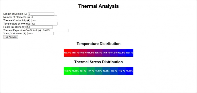
- 16 1D Thermal analysis using web based Java script:
- 17 The 33 DAI5 Implementation Evaluation Criteria
Predicting Static Stress in One-Dimensional Bar Elements Using Artificial Neural Networks coupled with DAI5 Framework-by-TanveeKhan
The given video is the part-1
The given video is the part-2
The 33 DAI5 Implementation Evaluation Criteria for Final project
Final_Term_Predicting Static Stress in One-Dimensional S275 J0 Bar Elements Using Artificial Neural Networks Coupled with DAI5 Framework
Tanveer Khan
Department of Mechanical Engineering, Faculty of Engineering, Universitas Indonesia, Kampus UI Depok, 16424, Indonesia
Abstract
This study introduces a novel approach for static stress prediction in one-dimensional bar elements having material composition S275 J0 by applying Artificial Neural Networks (ANNs) integrated with the Deep Awareness of I (DAI5) framework. The research focuses on developing a computationally efficient ANN model trained on FEM-generated data to predict stress under static loading conditions. The ANN architecture consists of two inputs (force and cross-sectional area), a single hidden layer with eight neurons, and one output layer to predict tensile stress. The 'logsig' activation function and Bayesian regularization were utilized to optimize model performance. Results indicate that the ANN predictions closely approximate FEM outcomes, with minimal error percentages across multiple test cases, validating the model's accuracy and reliability. Regression analysis demonstrates a high correlation coefficient (R=0.99998), confirming the ANN's robustness in generalizing patterns. The proposed ANN model offers significant advantages over traditional FEM in terms of computational speed and efficiency, making it suitable for real-time engineering applications and iterative simulations. Future extensions of this research include multi-dimensional stress analysis and applications to complex structural geometries.
Keywords: Static stress prediction, Artificial Neural Network (ANN), Deep Awareness of I (DAI5), One-dimensional bar elements, Finite Element Method (FEM), Tensile stress analysis, Computational efficiency
1. Author Declaration
1.1 Deep Awareness (of) I
The author’s conscious understanding of the role of self-awareness in this study is deeply rooted in the concept of Deep Awareness (of) I, which emphasizes a continuous remembrance of The One and Only, The Creator. This foundational principle highlights the interconnectedness of self-awareness and purposeful action. By fostering an awareness of the soul, the author aligns the research process with a higher intent serving not only technical goals but also fulfilling a spiritual purpose. In this context, the development of the ANN model and its integration with the DAI5 framework reflect a conscious pursuit of knowledge and truth, grounded in the remembrance of the Creator. The study becomes an act of alignment between intellectual exploration and spiritual understanding, ensuring that innovation is guided by ethical reflection and recognition of divine purpose.
1.2 Intention of Project Activity
The primary objective of this research is to develop and validate an advanced ANN model, augmented by the capabilities of the DAI5 framework, specifically tailored for predicting static stress within one-dimensional bar elements. This model aims to achieve a balance between accuracy and computational speed, thereby overcoming the inherent constraints associated with traditional finite element method (FEM) while ensuring consistency and reliability across diverse structural conditions. The study will focus on enhancing the ANN model's predictive capabilities by inputting critical parameters such as the magnitude and direction of applied loads, essential material property like Young’s modulus, geometric details including the bar's length and cross-sectional area, number of elements over the entire length of the bar, and one fixed node. Out of them, only the two inputs are variables such as cross-sectional area and applied force; the others are constant. Additionally, the integration of domain-specific insights through the DAI5 framework aims to significantly refine the model’s performance. Ultimately, this research endeavors to develop a reliable, efficient, and scalable predictive tool that seamlessly integrates into existing engineering processes, reducing the resources and time required for static stress analysis in one-dimensional bar elements. This innovation is poised to not only benefit professionals in the engineering field but also provide substantial advantages to local communities by enhancing the safety and durability of structural designs. This ultimately reduces costs and time for both local communities and the government. A well-designed structure is sustainable and requires less frequent maintenance and repairs, thereby saving time and money while also minimizing the risk of injuries and other hazards.
2. Introduction
There are various ways to approach the problem, however, Deep Awareness (of) I (DAI5) conscious thinking framework integrates philosophical self-awareness and intentional thinking into problem-solving, beginning with Dr. Ahmad Indra's concept of "I am My Consciousness." Unlike traditional methods that focus primarily on logical, step-by-step approaches, DAI5 emphasizes reflective consciousness at each stage: Intention (purpose) both technical and non-technical, Initial thinking about the problem (open brainstorming), Idealization (envisioning the best outcomes) simply the problem, and Instruction set (actionable steps). This approach differs by promoting deep self-awareness, ethical reflection, and holistic engagement, fostering solutions that align personal values with practical execution, rather than focusing solely on technical or analytical solutions. The first three I’s cover the author declaration and introduction of the manuscript and the remaining two I’s cover the methodology[1].
2.1 Initial thinking
There are various ways to perform stress analysis in FEM such as 1D elements analysis, 2D elements analysis, and 3D elements analysis. 1D elements are simpler and computationally less intensive compared to 2D and 3D elements. They are particularly useful for structures that can be approximated as beam-like, such as vehicle frames or I-beam[2]. These elements are often used in scenarios where the geometry of the structure is relatively simple, and the primary interest is in the overall behavior rather than detailed local effects. For example, they are commonly used in the automotive industry for simplified vehicle structure models[3]. Simplified 1D models, such as 1D-bar and 1D-beam models, are used for stress analysis in bonded joints. These models assume a linear elastic adhesive material and can simulate the entire bonded overlap using a four-node macro-element. These models can be extended to include elasto-plastic adhesive material behavior, providing results comparable to more complex 3D models[4]. Low-order displacement-based finite elements, such as 3-node and 4-node elements, are computationally efficient and can achieve good stress convergence in 1D solutions and a novel procedure improves stress predictions by ensuring that stress convergence is quadratic, matching the order of displacement convergence[5]. A method for steady-state viscoelastic stress analysis using FEM is described, which includes a one-dimensional case. This method is effective for calculating stress distribution and deformation in viscoelastic materials[6]. Classical 6-DOF beam theories, such as Euler-Bernoulli and Timoshenko, are evaluated for their accuracy in predicting higher-order phenomena like elastic bending/shear coupling and torsional warping. These theories are often used in 1D finite element models[7]. A refined 1D formulation for fiber-reinforced laminated composites allows for detailed stress/strain field descriptions by increasing the order of the 1D model. This approach provides accurate displacement/stress fields with low computational costs[8].
A 1D round bar, commonly referred to as a cylindrical or round bar, is a long, solid cylindrical piece of metal or alloy used in various industrial applications. These bars are integral in numerous sectors due to their mechanical properties and versatility. Round bars are used in the manufacturing of various components due to their strength and durability[9]. They serve as reinforcement in concrete structures and are used in the production of steel rebar[10]. Round bars are essential in producing machine parts, mechanical equipment, and seamless pipes for the oil and gas industry[11]. They are used in the production of components requiring high dimensional accuracy and specific mechanical properties[12]. They are made from various materials such as steel, aluminum, and alloys etc. Steel known for its excellent corrosion resistance and strength, steel round bars are widely used in construction and mechanical engineering[11]. Aluminum bars are preferred for applications requiring lightweight and nearly straight bars with minimal deformation[9]. Various alloys, such as 32CrB4 steel and AA 2219, are used for specific applications requiring high strength and specific mechanical properties[13, 14]. The mechanical properties of round bars, such as yield strength, tensile strength, and hardness, vary depending on the material and manufacturing process. For instance, AA 2219 alloy bars exhibit yield strengths of 288–304 MPa and tensile strengths of 410–428 MPa after T6 temper heat treatment[14]. Shape Memory Alloys (SMAs) round bars are designed to replace conventional steel bars in structural applications, offering super elasticity and shape memory effects[15]. Moreover, the strength of a round bar is affected by its diameter, with larger diameters generally showing different mechanical properties compared to smaller ones. For instance, larger diameter bars may exhibit higher tensile strength due to the increased volume of material resisting deformation[16, 17]. The mechanical properties of round bars, including yield strength, can be influenced by processing conditions such as drawing and straightening. Larger diameter bars may experience more significant changes in yield strength due to these processes[18, 19]. The bending stiffness of a round bar is directly related to its diameter. Larger diameter bars are stiffer and less prone to bending under load, whereas smaller diameter bars are more flexible and can bend more easily[20, 21]. The bending strength of round bars can be affected by the presence of defects or initial damage, which is more pronounced in larger diameter bars due to the higher stress concentrations[21, 22]. Residual stresses within the bar, which can be compressive or tensile, vary with diameter. Smaller diameter bars tend to have compressive stresses, while larger diameter bars may exhibit tensile stresses, impacting their overall strength[23].
S275 J0 is a grade of structural steel that falls under the S275 category, which is a popular low carbon steel used in various engineering and structural applications. This type of steel is widely utilized in construction, maintenance, machinery, and manufacturing industries due to its favorable mechanical properties and weldability. It exhibits a combination of mechanical properties that make it suitable for structural applications such as the yield strength typically around 275 MPa, which is a standard requirement for this grade of steel, and the tensile strength ranges from 410 to 560 MPa, providing adequate strength for various structural applications[24]. The steel's properties make it suitable for use in bridge construction, where it can handle significant loads and stresses, besides that the 'J0' designation indicates that the steel has been tested for impact resistance at 0°C, ensuring its performance in moderately cold environments[25]. Its good weldability makes it an excellent choice for welded beams and columns in various structural applications, and it is relatively inexpensive compared to higher-grade steels, making it a cost-effective choice for many construction projects [26]
Artificial Neural Networks (ANNs) have emerged as powerful tools for structural stress analysis, offering efficient alternatives to traditional methods like finite element analysis (FEA). These models leverage machine learning techniques to predict stress distributions and responses under various loading conditions, significantly reducing computational costs and time, Machine learning (ML) has shown significant promise in the field of structural stress analysis, offering innovative solutions to traditional challenges, ML techniques have been employed to expedite the multiscale analysis of composite materials. By learning the relationships between different scales, ML models can significantly reduce computation times while maintaining high accuracy in stress predictions[27]. Artificial Neural Networks (ANNs) have been applied to improve stress recovery in FEA. Traditional FEA often provides accurate stress values only at specific points (super-convergent points. ANNs can map the stress field across the entire domain, enhancing accuracy and efficiency[28]. ML algorithms have been used to estimate axial stress in CWR by analyzing vibration data. By training ML models with data from finite element models, researchers can predict stress from vibration frequencies, demonstrating ML's viability in real-world applications[29]. Various ML models, including Gaussian Process Regression (GPR), Neural Networks (NN), and Boosted Trees (BST), have been used to predict stress-strain curves for materials like aluminum alloys. These models have shown high accuracy, with NNs achieving a coefficient of determination (R²) of 0.998[30]. ML models can provide highly accurate predictions, often surpassing traditional empirical models. For example, gradient boosting models have shown superior prediction accuracy for flow stress in high entropy alloys[31]. An Artificial Neural Network (ANN) is utilized to establish the relationship between selected feature elements and correlation elements for structural stress analysis. This approach enhances accuracy in measuring global stress in marine structures, achieving 93.6% accuracy in real-scale model tests[32].
Prediction, also known as forecasting, is a fundamental task across various scientific and engineering disciplines. It involves estimating outcomes based on past data and observed patterns. There are various models to predict the outcomes. Firstly, statistical methods including; Linear Regression used to predict values based on the relationship between dependent and independent variables[33], Logistic Regression commonly used for binary classification tasks[34], Naïve Bayes a probabilistic classifier based on Bayes' theorem[34], and Decision Trees a model that splits data into branches to make predictions[34]. Secondly, machine learning algorithms such as; Support Vector Machines (SVM) effective for classification and regression tasks[35], Artificial Neural Networks (ANN) used for complex pattern recognition and prediction tasks[36], and K-Nearest Neighbors (KNN) a simple, instance-based learning algorithm[34]. Lastly, Deep Learning Methods comprise of; Multilayer Perceptron (MLP) a type of neural network used for time series prediction and other tasks[37], and Deep Learning Models employed for handling large datasets and complex prediction tasks[38]. In the context of stress prediction, FEA is widely used to predict static stress by simulating the stress-strain response of materials under various loading conditions. This method can be enhanced by data-driven models to improve accuracy[39]. ANNs can be trained using displacement and force data to predict the stress state of materials. This method leverages synthetic data from virtual experiments to enhance prediction accuracy[40].
2.2 Problem statement
The prediction of static stress in structural elements, such as one-dimensional bar elements, remains a computationally intensive task when relying on traditional Finite Element Methods (FEM). While FEM offers precise stress distribution analysis, its high computational cost and time requirements pose significant limitations, especially for large-scale or iterative simulations in real-time engineering applications. Additionally, the simplification of geometric configurations, like one-dimensional bar elements, often leads to challenges in balancing accuracy and efficiency. The need for a scalable, accurate, and computationally efficient alternative has become increasingly critical in structural analysis to optimize resources and enhance engineering workflows. This study addresses the gap by proposing an Artificial Neural Network (ANN) model, augmented with the Deep Awareness of I (DAI5) framework, as a surrogate to FEM. This innovative approach aims to overcome the computational challenges while ensuring robust and accurate predictions of static tensile stress under varying input conditions, thus providing a cost-effective and time-saving solution for engineers and designers.
3. Methodology
3.1 Idealization
3.1.1 Material
Mild steel is widely used in structural applications due to its favorable mechanical properties, affordability, and versatility. Among its various grades, S275 J0 is extensively employed in structural components, offering an optimal combination of strength, ductility, and weldability. This study focuses on predicting the static tensile stress of S275 J0 under static loading conditions using an Artificial Neural Network (ANN). To train the ANN's, the Finite Element Method (FEM) is incorporated for generating reliable training data to feed the ANN. This integration ensures to avoid experiments data collection. The mechanical properties of S275 J0 are presented in (Table 1)[41].
2.1.2 Finite Element Method (FEM)
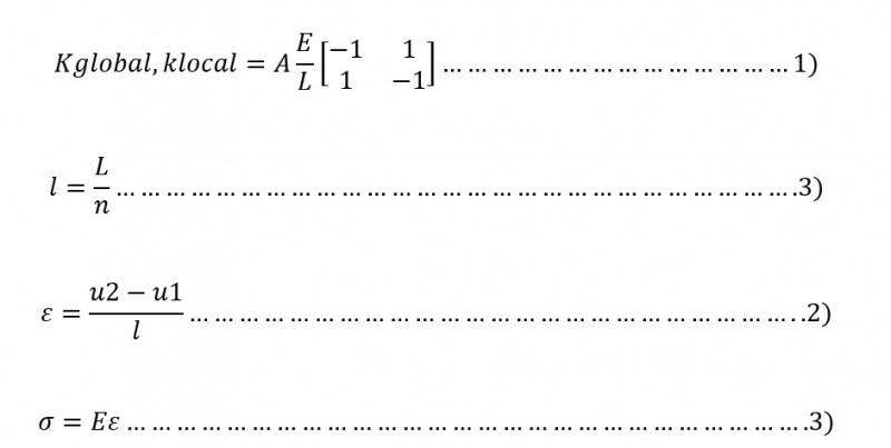
The Finite Element Method (FEM) is a powerful numerical technique used to obtain approximate solutions to a wide range of engineering problems, and is used to solve partial differential equations (PDEs) with specific boundary conditions by discretizing the solution region into smaller, simpler parts called finite elements, which can be assembled in various ways to represent complex shapes[42]. There are various ways to conduct finite element analysis to predict stress in a bar such as 1D, 2D, and 3D. However, 1D is simpler one, and the discrete elements are typically line segments[43]. Using one-dimensional elements allows for a straightforward mathematical description, making it easier to understand the principles and assumptions of mechanical modeling without complex mathematics[44]. The following 1D equations (1,2,3)[45] we used in our study for the predict of static stress in the bar.
Where:
K= Stiffness matrix.
E = Young's modulus of the material (Pa).
A = Cross-sectional area of the bar (m^2).
L =Length of the bar (m).
n= number of elements to divide the bar into.
l= element length (m).
u2-u1= change in length of the element (m).
ε= strain (m).
σ= stress (Pa).
2.1.3 Artificial neural network (ANN)
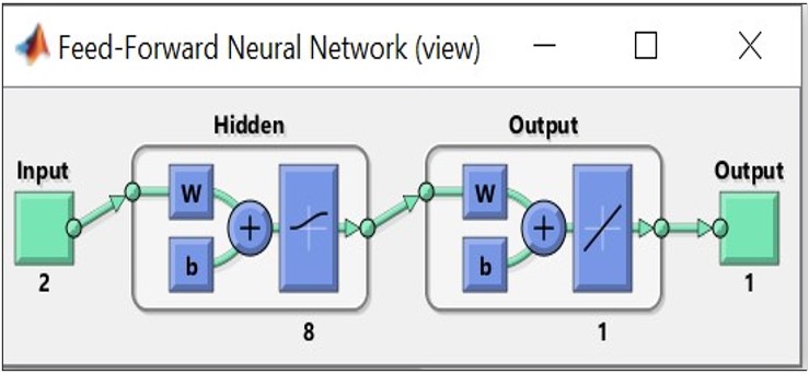
The architecture of an ANN typically includes an input layer, one or more hidden layers, and an output layer. The number of hidden layers and the number of neurons in each layer are crucial parameters. An optimal configuration balances complexity and performance, avoiding underfitting or overfitting[46]. The choice of activation function (e.g. ReLU, logsig) affects how the network learns and processes information. Different functions can be applied to different layers to enhance performance[47]. Based on simplicity and performance considerations, the following Artificial Neural Network (ANN) configuration was applied using MATLAB to predict the static tensile stress in a bar. The ANN model utilized two inputs (the cross-sectional area and the applied force) both of which are critical parameters influencing tensile stress. A single hidden layer with 8 neurons was chosen to balance computational efficiency and model accuracy. The output layer predicted the tensile stress of the bar, which serves as the primary objective of this analysis. To ensure optimal performance, the ‘logsig’ activation function was used. This activation function demonstrated superior results in comparison to other alternatives based on a trial-and-error method, where the primary evaluation criteria included computational time, performance (mean squared error), and the correlation coefficient (R) between predicted and actual values. The ‘logsig’ activation function is advantageous for its smooth, nonlinear properties, which allow the ANN to approximate complex relationships between inputs and outputs effectively. This configuration strikes a balance between model simplicity and prediction accuracy, making it suitable for real-time applications and structural analysis tasks. The study demonstrates that integrating this ANN configuration can provide reliable predictions of tensile stress, thereby offering an efficient alternative to traditional methods like direct FEM simulations.
2.2 Instructure set
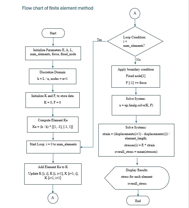
2.2.1 Finite element method
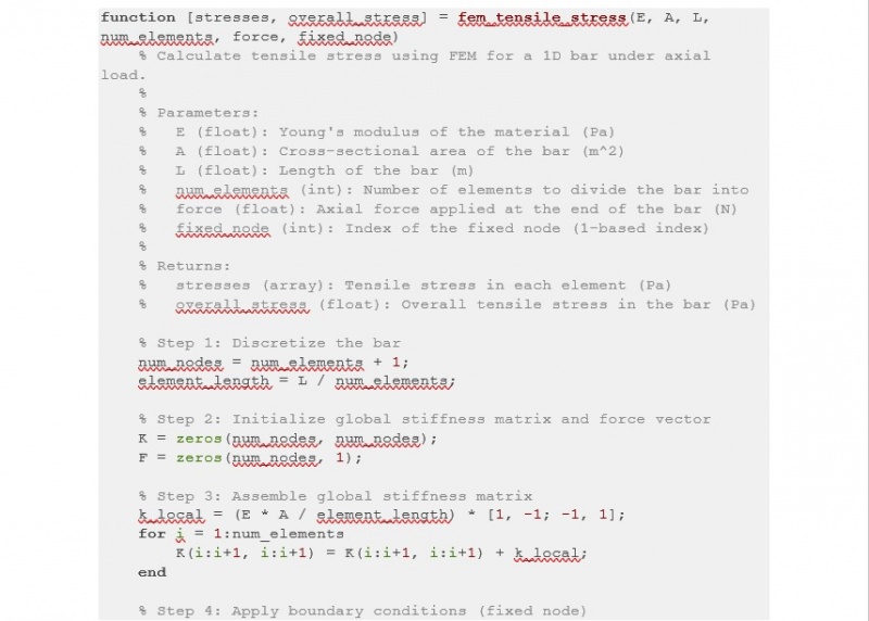
Step 1: Input Data to the model using MATLAB R2018a
Provide material properties, geometry, and load.
E =Young's modulus (Pa).
A=Cross-sectional area (m²).
L=Total bar length (m).
num_elements=Number of finite elements.
force=Axial force applied at the free end (N).
fixed_node=Fixed node index.
Step 2: Discretization
Divide the bar into num_elements segments.
Calculate the length of each element form the equation l=L/n.
Define the number of nodes from the equation num_nodes=num_elements+1.
Step 3: Global Stiffness Matrix Assembly
Initialize a global stiffness matrix K of size (num_nodes x num_nodes).
Define the local stiffness matrix for an element k(local)=A E/L [[-1 1]; [1 -1]].
Loop over each element and add the local stiffness matrix to the global stiffness matrix K.
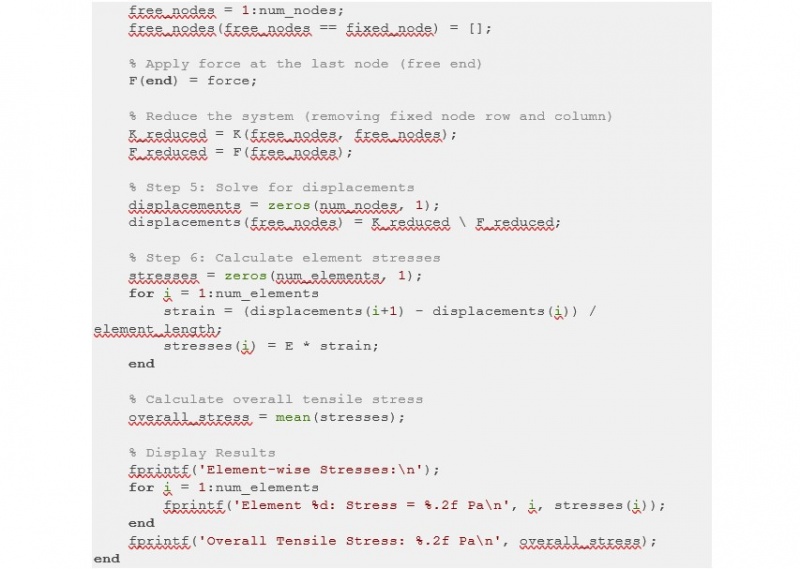
Step 4: Apply Boundary Conditions
Fix the specified node (fixed_node) by eliminating the corresponding row and column in K.
Apply the force at the last node such as 𝐹end=force. Modify the system to exclude the fixed node.
Step 5: Solve for Displacements
Solve the reduced system of equations: K (reduced) x u (free)=F (reduced)where u (free) are the unknown displacements at free nodes.
Add the solved displacements back into the displacement vector u, including a zero displacement for the fixed node.
Step 6: Calculate Element Stresses
Compute strain in each element using ε=(u2-u1)/l.
Calculate element stress using Hooke's law as σ=Eε.
Store stresses for all elements.
Step 7: Compute Overall Stress and Display Results
Average the element stresses to find the overall tensile stress as overall_stress=mean(stresses)
Print the stress for each element and the overall tensile stress.
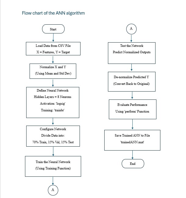
2.2.2 Artificial neural network ANN
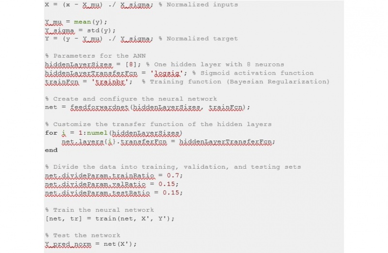
Step 1: Load Data to the MATLAB R2018a
Load data from a CSV file ().
Extract X as Features (input data) from columns and Y as Target values (output data) from column.
Step 2: Normalize Data
Normalize the inputs X and targets Y using mean (μ) and standard deviation (σ).
Step 3: Define Neural Network Architecture
Choose parameters for the ANN such as number of layers (One hidden layer with 8 neurons).
Activation function like logsig for the hidden layer.
Training function using Bayesian Regularization (trainbr).
Create the neural network using net=feedforwardnet(hiddenLayerSizes, trainFcn).
Step 4: Configure Neural Network
Update the transfer function for hidden layers using Matlab code net.layers{i}.transferFcn = 'logsig';
Divide data into. Such as 70% Training, 15% Validation, and 15% for Testing.
Step 5: Train the Neural Network
Use the training function to train the network using the code line [net,tr]=train(net, X’, Y’).
Step 6: Test the Network
Predict normalized outputs using the trained network such as Y pred_norm=net(Xt ).
Denormalize predictions back to the original scale by using the code line Y pred=(Y pred_norm *Yσ)+Yμ.
Step 7: Calculate Performance
Evaluate network performance using the performance function=perform(net, Y’, Y_pred).
Step 8: Save Trained Network
Save the trained network to a .mat file using code save('trainedANN.mat', 'net')
4. Results and discussion
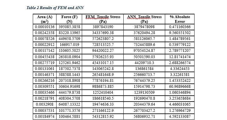
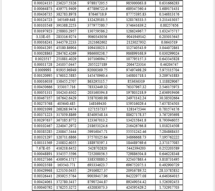
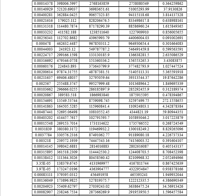
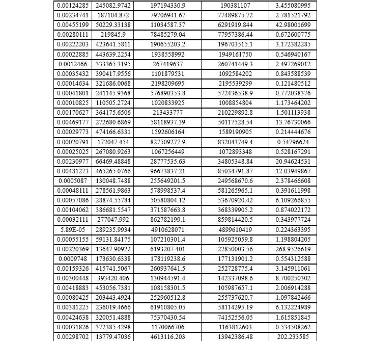
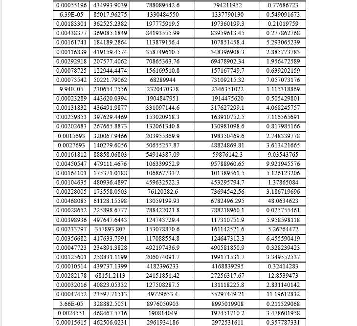
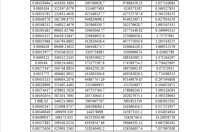
The (Table 2) presents predicted tensile stress values from the ANN model alongside FEM results. It also includes the absolute percent error of ANN predictions, highlighting their accuracy. This comparison demonstrates the ANN's ability to approximate FEM outcomes, with minor deviations indicating the model's reliability for tensile stress prediction in engineering applications. The key parameters include the cross-sectional area A, applied force F, FEM-predicted tensile stress, ANN-predicted tensile stress, and the absolute percentage error between ANN and FEM results. The FEM results serve as a benchmark for tensile stress prediction, while ANN results approximate these values based on training and generalization capabilities. The absolute percentage error varies across the cases. For instance, in the first case, the error is minimal at 0.47%, indicating high alignment between ANN and FEM predictions. The second case exhibits a larger error of 9.56%, suggesting some deviation, likely due to nonlinearities or ANN training limitations. For the remaining cases, errors generally stay within a small range (0.5%-2.8%), demonstrating that ANN predictions are close to FEM results. Smaller errors (0.47%, 0.54%) suggest that the ANN effectively learns from the input-output relationships for tensile stress. Larger deviations, as seen in case 2, may arise when input values fall outside the ANN’s training range or involve variations that the model could not fully capture. The ANN model achieves reasonably accurate predictions of tensile stress, with absolute errors mostly below 3%. These small deviations validate the ANN’s reliability for estimating FEM results, offering computational efficiency and reduced processing time compared to FEM, particularly for iterative simulations. The findings demonstrate that ANN models can effectively approximate FEM results in tensile stress prediction, making them valuable tools for engineering applications where rapid predictions are required.
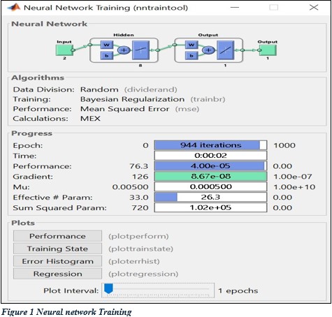
The (Figure 1) shows the Neural Network Training (nntraintool) interface for an Artificial Neural Network (ANN) model trained using Bayesian Regularization (trainbr). The neural network comprises 2 inputs, 1 hidden layer with 8 neurons, and 1 output. The network completed 944 iterations out of the 1000 iterations allowed, showing it approached convergence early. Training lasted 2 seconds, demonstrating computational efficiency due to the network’s simple architecture. The performance achieved is 4.00e-05, which is a very small error. This indicates that the network closely approximates the target values, confirming high accuracy. The gradient value is 8.67e-08, which is near zero. A low gradient suggests that the training process has reached an optimal solution where weight adjustments are minimal.The parameter μ remains constant at 0.005, indicating stable Bayesian regularization without divergence or instability. The network uses approximately 26.3 effective parameters out of 33, demonstrating efficiency in parameter utilization and avoiding overfitting.
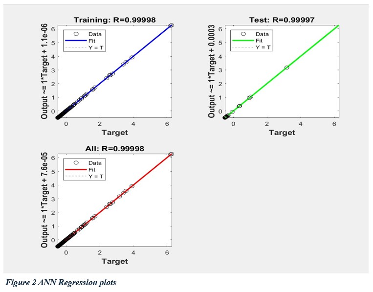
The (Figure 2) presents regression plots for the training, testing, and overall performance of the Artificial Neural Network (ANN) used to predict tensile stress. These plots demonstrate the relationship between the target values (actual data) and the network outputs (predicted values) for different phases of training. The regression coefficient R, which indicates the linear correlation between the ANN outputs and targets, is provided for each phase. In the top-left plot, the regression coefficient for the training set is R=0.99998, indicating an almost perfect correlation between the ANN predictions and the actual target values. The blue line, representing the best fit, closely aligns with the diagonal line Y=T, where the output equals the target. The very slight offset (1.1 × 10⁻⁶) confirms minimal prediction error. This near-perfect regression demonstrates that the network effectively learned the underlying patterns in the training data, achieving high accuracy. The clustering of data points along the ideal line further supports the strong generalization of the model within the training phase. The top-right plot shows the performance of the ANN on the testing set, with R=0.99997. The regression coefficient remains close to 1.0, indicating excellent agreement between predictions and actual targets for unseen data. The green fitting line also aligns well with the Y=T line, with a minor offset of 0.0003. This small deviation highlights the ANN’s robustness and ability to generalize its learned patterns to new, unseen data. The consistency between training and testing results suggests that overfitting has been avoided, a notable achievement given the complexity of neural network training. The bottom plot combines all the data (training, validation, and testing) and reports an overall regression coefficient of R=0.99998. The red fit line closely follows the Y=T line, with an extremely small offset of 7.6×10⁻⁵ .This result further confirms the model's excellent performance across the entire dataset. The high R-value indicates a strong linear correlation between the predicted and actual tensile stress values, underscoring the ANN's reliability and precision.
The regression results collectively demonstrate the high predictive accuracy of the ANN model. The near-perfect R-values across training, testing, and overall phases confirm the network’s ability to approximate the FEM results with minimal errors. The consistency of performance across the subsets of data is particularly significant, as it indicates that the network has successfully generalized its predictions without overfitting or underfitting. From a practical perspective, the results highlight the ANN's capability to serve as a reliable surrogate model for tensile stress prediction. Traditional methods such as Finite Element Analysis (FEA) are computationally expensive and time-consuming, especially for large-scale or iterative simulations. The ANN model, on the other hand, provides rapid and accurate predictions, making it highly suitable for real-time engineering applications where efficiency is paramount. Furthermore, the minimal offsets observed in the regression lines suggest that the ANN is capable of handling noise or variations in input data without significant loss of accuracy. This robustness is a critical factor in practical implementations where real-world data often contains inherent variability.
5. Conclusion
The integration of Artificial Neural Networks (ANN) with the Finite Element Method (FEM) has proven to be a highly effective approach for static stress prediction in one-dimensional bar elements. By leveraging the DAI5 framework, this study has successfully demonstrated a novel methodology that balances computational efficiency with predictive accuracy. The ANN model showcased high alignment with FEM results, achieving minimal prediction errors, which underscores its potential as a reliable surrogate for FEM in engineering applications. Moreover, the ANN's ability to generalize across diverse input scenarios highlights its robustness and adaptability for real-world use. These findings validate the ANN's applicability in reducing computational costs and expediting stress analysis processes, particularly in iterative simulations and large-scale engineering tasks.
Future research should explore applying this ANN-based framework to multi-dimensional stress analysis and more complex geometries, broadening its usability across various structural engineering scenarios.
6. Acknowledgments
The author gratefully acknowledges the support and contributions provided by Universitas Indonesia for facilitating this research. Special thanks are extended to the Department of Mechanical Engineering, Faculty of Engineering, for their resources and guidance throughout the study. The author also wishes to express gratitude to mentors whose insights and encouragement have significantly enriched the research process.
7. References
[1] D. A. Indra. "Deep Awareness (of) I (DAI5) Framework." https://air.eng.ui.ac.id/index.php?title=Main_Page (accessed.
[2] C. M. Wai, A. Rivai, and O. Bapokutty, "Modelling optimization involving different types of elements in finite element analysis," in IOP Conference Series: Materials Science and Engineering, 2013, vol. 50, 1 ed., doi: 10.1088/1757-899X/50/1/012036. [Online]. Available: https://www.scopus.com/inward/record.uri?eid=2-s2.0-84893574266&doi=10.1088%2f1757-899X%2f50%2f1%2f012036&partnerID=40&md5=f1f018e49b16a62d4e13fc279deb1527
[3] P. Mihaylova, N. Baldanzini, and M. Pierini, "Considerations on 1D beam concept modelling for the vehicle structure," in International Conference on Noise and Vibration Engineering 2012, ISMA 2012, including USD 2012: International Conference on Uncertainty in Structure Dynamics, 2012, vol. 5, pp. 3793-3808. [Online]. Available: https://www.scopus.com/inward/record.uri?eid=2-s2.0-84906330927&partnerID=40&md5=14669964066ea29b3d1fdf60b455df5b. [Online]. Available: https://www.scopus.com/inward/record.uri?eid=2-s2.0-84906330927&partnerID=40&md5=14669964066ea29b3d1fdf60b455df5b
[4] E. Paroissien, F. Gaubert, A. Da Veiga, and F. Lachaud, "Elasto-plastic analysis of bonded joints with macro-elements," Journal of Adhesion Science and Technology, Article vol. 27, no. 13, pp. 1464-1498, 2013, doi: 10.1080/01694243.2012.745053.
[5] D. J. Payen and K. J. Bathe, "A stress improvement procedure," Computers and Structures, Article vol. 112-113, pp. 311-326, 2012, doi: 10.1016/j.compstruc.2012.07.006.
[6] F. Qin, Y. Yu, and T. Rudolphi, "Finite element modeling of viscoelastic stress analysis under moving loads," World Academy of Science, Engineering and Technology, Article vol. 50, pp. 941-948, 2011. [Online]. Available: https://www.scopus.com/inward/record.uri?eid=2-s2.0-84871277457&partnerID=40&md5=2cad14132cbf04614b57759b670dbbef.
[7] E. Carrera and A. Pagani, "Evaluation of the accuracy of classical beam FE models via locking-free hierarchically refined elements," International Journal of Mechanical Sciences, Article vol. 100, pp. 169-179, 2015, doi: 10.1016/j.ijmecsci.2015.06.021.
[8] E. Carrera, M. Maiarú, M. Petrolo, and G. Giunta, "A refined 1D element for the structural analysis of single and multiple fiber/matrix cells," Composite Structures, Article vol. 96, pp. 455-468, 2013, doi: 10.1016/j.compstruct.2012.09.012.
[9] S. Roy and A. K. Pal, "A novel approach for study of straightness in commercially produced round metal bars based on deflection measurements," Applications in Engineering Science, Article vol. 16, 2023, Art no. 100161, doi: 10.1016/j.apples.2023.100161.
[10] V. N. Shinkin, "Elastoplastic Flexure of Round Steel Beams. 1. Springback Coefficient," Steel in Translation, Article vol. 48, no. 3, pp. 149-153, 2018, doi: 10.3103/S0967091218030117.
[11] V. N. Shinkin, "Elastoplastic bend of round steel beam. Report 1. springback coefficient," Izvestiya Ferrous Metallurgy, Article vol. 61, no. 3, pp. 194-200, 2018, doi: 10.17073/0368-0797-2018-3-194-200.
[12] M. Asakawa, "Part 1: Trends in drawing technology for bars and wires," Wire Journal International, Article vol. 47, no. 8, pp. 60-66, 2014. [Online]. Available: https://www.scopus.com/inward/record.uri?eid=2-s2.0-84940307389&partnerID=40&md5=583a4dbbc1bc0dd040b183bc2f2e527a.
[13] A. Stepanov, A. Koldaev, N. Arutyunyan, and A. Zaitsev, "Evolution of the Structural State and Properties of 32CrB4 Steel during the Production of High-Strength Fasteners," Metals, Article vol. 12, no. 2, 2022, Art no. 366, doi: 10.3390/met12020366.
[14] T. R. Prabhu, "Effects of ageing time on the mechanical and conductivity properties for various round bar diameters of AA 2219 Al alloy," Engineering Science and Technology, an International Journal, Article vol. 20, no. 1, pp. 133-142, 2017, doi: 10.1016/j.jestch.2016.06.003.
[15] M. K. Song, E. Choi, and J. H. Lee, "Development and Performance Evaluation of a Mechanical Connection for Steel and Shape Memory Alloy Bars," Metals, Article vol. 14, no. 3, 2024, Art no. 300, doi: 10.3390/met14030300.
[16] J. Gu, "Approach to mechanical properties of die casting components," Tezhong Zhuzao Ji Youse Hejin/Special Casting and Nonferrous Alloys, Article vol. 25, no. 8, pp. 482-484, 2005. [Online]. Available: https://www.scopus.com/inward/record.uri?eid=2-s2.0-24744466912&partnerID=40&md5=6ca5341ac775ffbfc7c593a004369d63.
[17] "Experimental investigation on bond of largediameter reinforcing bars," in fib Bulletins, vol. 2022, 2022, pp. 98-109.
[18] B. Rivolta, G. Silva, M. Rota, and M. Cusolito, "Drawn bars: Influence of straightening conditions," Wire Journal International, Article vol. 37, no. 5, pp. 77-81, 2004. [Online]. Available: https://www.scopus.com/inward/record.uri?eid=2-s2.0-2542513096&partnerID=40&md5=713de22f81aadc388850dbc1795be450.
[19] Y. Tanaka, M. Asakawa, R. Komami, and H. Kubota, "Effect of mechanical properties on diameter of drawn bars," Wire Journal International, Article vol. 42, no. 11, pp. 66-71, 2009. [Online]. Available: https://www.scopus.com/inward/record.uri?eid=2-s2.0-71949101522&partnerID=40&md5=21558bbad821a3a1f816b6015e90056d.
[20] Y. Song, Z. Guan, Y. Nie, and X. Guan, "The analysis of the bending stiffness and intensity of cylindrical tubes," Science in China, Series E: Technological Sciences, Article vol. 50, no. 3, pp. 268-278, 2007, doi: 10.1007/s11431-007-0031-3.
[21] Y. L. Zheng, Y. T. Sun, H. R. Lin, J. Q. Wang, X. Liu, and C. H. Lu, "Experimental study of initial damage to steel bars due to bending process and the resulting performance deterioration," Construction and Building Materials, Article vol. 411, 2024, Art no. 134326, doi: 10.1016/j.conbuildmat.2023.134326.
[22] Y. Zheng, X. Liu, C. Lu, S. Bu, and K. Kosa, "Incipient Damage When Bending Stirrup and Its Influence on Mechanical Properties," Cailiao Daobao/Materials Reports, Article vol. 36, no. 23, 2022, Art no. 21110130, doi: 10.11896/cldb.21110130.
[23] G. Roy and K. Sennah, "Residual stress in axisymmetric rods," in AES-ATEMA International Conference Series - Advances and Trends in Engineering Materials and their Applications, 2009, pp. 111-117. [Online]. Available: https://www.scopus.com/inward/record.uri?eid=2-s2.0-84856622647&partnerID=40&md5=e2570fdb937b225a08b45d08a56e2bd7. [Online]. Available: https://www.scopus.com/inward/record.uri?eid=2-s2.0-84856622647&partnerID=40&md5=e2570fdb937b225a08b45d08a56e2bd7
[24] B. Çevik, "Effect of welding processes on mechanical and microstructural properties of S275 structural steel joints," Materialpruefung/Materials Testing, Article vol. 60, no. 9, pp. 863-868, 2018, doi: 10.3139/120.111225.
[25] J. Brnic, G. Turkalj, J. Niu, M. Canadija, and D. Lanc, "Analysis of experimental data on the behavior of steel S275JR - Reliability of modern design," Materials and Design, Article vol. 47, pp. 497-504, 2013, doi: 10.1016/j.matdes.2012.12.037.
[26] T. Lipiński, "Corrosion of S235JR steel in NaCL environment at 3 °c," in METAL 2017 - 26th International Conference on Metallurgy and Materials, Conference Proceedings, 2017, vol. 2017-January, pp. 660-665. [Online]. Available: https://www.scopus.com/inward/record.uri?eid=2-s2.0-85043327383&partnerID=40&md5=bbfb99a56487675d5bce750b42101320. [Online]. Available: https://www.scopus.com/inward/record.uri?eid=2-s2.0-85043327383&partnerID=40&md5=bbfb99a56487675d5bce750b42101320
[27] W. Kuś, W. Mucha, and I. T. Jiregna, "Multiscale Analysis of Composite Structures with Artificial Neural Network Support for Micromodel Stress Determination," Materials, Article vol. 17, no. 1, 2024, Art no. 154, doi: 10.3390/ma17010154.
[28] B. B. Saikia, D. Nath, and S. S. Gautam, "Application of machine learning in efficient stress recovery in finite element analysis," in Materials Today: Proceedings, 2023, vol. 78, pp. 359-363, doi: 10.1016/j.matpr.2022.10.100. [Online]. Available: https://www.scopus.com/inward/record.uri?eid=2-s2.0-85141385166&doi=10.1016%2fj.matpr.2022.10.100&partnerID=40&md5=175dba8b506c4c8801ab5e7ff3c87e2b
[29] M. Belding, A. Enshaeian, and P. Rizzo, "A Machine learning-based approach to determining stress in rails," Structural Health Monitoring, Article vol. 22, no. 1, pp. 639-656, 2023, doi: 10.1177/14759217221085658.
[30] A. Dorbane, F. Harrou, D. C. Anghel, and Y. Sun, "Machine Learning Prediction of Aluminum Alloy Stress–Strain Curves at Variable Temperatures with Failure Analysis," Journal of Failure Analysis and Prevention, Article vol. 24, no. 1, pp. 229-244, 2024, doi: 10.1007/s11668-023-01833-2.
[31] S. K. Dewangan et al., "Enhancing flow stress predictions in CoCrFeNiV high entropy alloy with conventional and machine learning techniques," Journal of Materials Research and Technology, Article vol. 30, pp. 2377-2387, 2024, doi: 10.1016/j.jmrt.2024.03.164.
[32] T. Zhang et al., "Reconstructing the Global Stress of Marine Structures Based on Artificial-Intelligence-Generated Content," Applied Sciences, vol. 13, no. 14, doi: 10.3390/app13148196.
[33] Y. Mishra, S. Mishra, and P. K. Mallick, "A Regression Approach Towards Climate Forecasting Analysis in India," in Lecture Notes in Networks and Systems, 2022, vol. 375, pp. 457-465, doi: 10.1007/978-981-16-8763-1_37. [Online]. Available: https://www.scopus.com/inward/record.uri?eid=2-s2.0-85132028355&doi=10.1007%2f978-981-16-8763-1_37&partnerID=40&md5=296facd8681f403b4c78711986db19f2
[34] T. Goswami, "Machine learning behind classification tasks in various engineering and science domains," in Cognitive Informatics, Computer Modelling, and Cognitive Science: Volume 1: Theory, Case Studies, and Applications, 2020, pp. 339-356.
[35] D. Liu, Y. Peng, and X. Peng, "Online adaptive status prediction strategy for data-driven fault prognostics of complex systems," in 2011 Prognostics and System Health Management Conference, PHM-Shenzhen 2011, 2011, doi: 10.1109/PHM.2011.5939530. [Online]. Available: https://www.scopus.com/inward/record.uri?eid=2-s2.0-79960910267&doi=10.1109%2fPHM.2011.5939530&partnerID=40&md5=774d6ca54d55e118a78e63f216d0a1ee
[36] S. Han, T. Hong, G. Kim, and S. Lee, "Technical comparisons of simulation-based productivity prediction methodologies by means of estimation tools focusing on conventional earthmovings," Journal of Civil Engineering and Management, Article vol. 17, no. 2, pp. 265-277, 2011, doi: 10.3846/13923730.2011.574381.
[37] K. N. Myint and M. Khaing, "Time Series Forecasting System for Stock Market Data," in IEEE International Conference on Control and Automation, ICCA, 2023, vol. 2023-February, pp. 56-61, doi: 10.1109/ICCA51723.2023.10181945. [Online]. Available: https://www.scopus.com/inward/record.uri?eid=2-s2.0-85166283979&doi=10.1109%2fICCA51723.2023.10181945&partnerID=40&md5=f22632502068119381e416e3f453587a
[38] B. U. Maheswari, S. Kirubakaran, P. Saravanan, M. Jeyalaxmi, A. Ramesh, and R. G. Vidhya, "Implementation and Prediction of Accurate Data Forecasting Detection with Different Approaches," in Proceedings of the 4th International Conference on Smart Electronics and Communication, ICOSEC 2023, 2023, pp. 891-897, doi: 10.1109/ICOSEC58147.2023.10276331. [Online]. Available: https://www.scopus.com/inward/record.uri?eid=2-s2.0-85175695713&doi=10.1109%2fICOSEC58147.2023.10276331&partnerID=40&md5=fb8be12ce3e577f41c15d76b48ec9cc5
[39] X. Li, Z. Li, Y. Chen, and C. Zhang, "An enhanced data-driven constitutive model for predicting strain-rate and temperature dependent mechanical response of elastoplastic materials," European Journal of Mechanics, A/Solids, Article vol. 100, 2023, Art no. 104996, doi: 10.1016/j.euromechsol.2023.104996.
[40] R. Lourenço, A. Andrade-Campos, and P. Georgieva, "The Virtual Fields Method to Indirectly Train Artificial Neural Networks for Implicit Constitutive Modelling," in Key Engineering Materials, 2022, vol. 926 KEM, pp. 2060-2068, doi: 10.4028/p-gy2di7. [Online]. Available: https://www.scopus.com/inward/record.uri?eid=2-s2.0-85140455747&doi=10.4028%2fp-gy2di7&partnerID=40&md5=c1a33ebfdba66e5f99a233db5ff4e9a6
[41] D. McClements. "All About Mild Steel." https://www.xometry.com/resources/materials/mild-steel/ (accessed.
[42] V. Jagota, A. P. S. Sethi, and K. Kumar, "Finite element method: An overview," Walailak Journal of Science and Technology, Review vol. 10, no. 1, pp. 1-8, 2013. [Online]. Available: https://www.scopus.com/inward/record.uri?eid=2-s2.0-84884232632&partnerID=40&md5=978bc7ff76751fb4aadd81c407653ca2.
[43] A. Quarteroni, "Generation of 1D and 2D grids," in Modeling, Simulation and Applications, vol. 16, 2017, pp. 141-160.
[44] A. Öchsner and M. Merkel, One-dimensional finite elements: An introduction to the FE method (One-Dimensional Finite Elements: An Introduction to the FE Method). 2013, pp. 1-398.
[45] Y. Charles, "A finite element formulation to model extrinsic interfacial behavior," 2014, doi: 10.1016/j.finel.2014.05.008.
[46] W. Fink, "Autonomous self-configuration of artificial neural networks for data classification or system control," in Proceedings of SPIE - The International Society for Optical Engineering, 2009, vol. 7331, doi: 10.1117/12.821836. [Online]. Available: https://www.scopus.com/inward/record.uri?eid=2-s2.0-69949172844&doi=10.1117%2f12.821836&partnerID=40&md5=1a2160eec0d56383c7efc38b3368c127
[47] M. R. Shaeri, A. M. Randriambololona, and S. Sarabi, "Prediction Accuracy of Artificial Neural Networks in Thermal Management Applications Subject to Neural Network Architectures," in Proceedings of the World Congress on Mechanical, Chemical, and Material Engineering, 2022, doi: 10.11159/htff22.175. [Online]. Available: https://www.scopus.com/inward/record.uri?eid=2-s2.0-85145297886&doi=10.11159%2fhtff22.175&partnerID=40&md5=dad358820386a0405180e02837363f17
8. Appendices
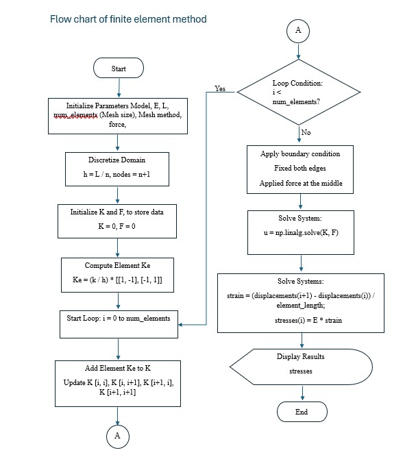
8.1 Finite element method algorithm
8.2 Artificial neural network algorithm
End of Final Term
Video_Mid_Term_Optimization of 2D Element Mesh in plane stress analysis of Polycarbonate Shell Structures Using the DAI5 Framework
Writing_Mid_Term_Optimization of 2D Element Mesh in plane stress analysis of Polycarbonate Shell Structures Using the DAI5 Framework
Tanveer Khan
Department of Mechanical Engineering, Faculty of Engineering, Universitas Indonesia, Kampus UI Depok, 16424, Indonesia
Abstract
This study investigates the optimization of 2D element mesh configurations in polycarbonate shell structures using the DAI5 conscious thinking Framework. Finite Element Analysis (FEA) methods were applied to analyze stress distributions in shell structures under static loading conditions. The goal is to identify the optimal mesh size and method for accurate stress analysis under plane stress conditions, focusing on three meshing techniques: Multizone Quad/Tri, Quadrilateral Dominant, and Triangle. Each technique was evaluated at varying mesh sizes (1 mm, 2 mm, and 3 mm) using ANSYS simulation software. Results indicate that the Multizone Quad/Tri method provides a balanced approach with high accuracy and computational efficiency at 2 mm mesh size. The Quadrilateral Dominant method demonstrated consistent accuracy across different mesh sizes but with slightly longer computation times. The Triangle method yielded the most detailed stress analysis but at a higher computational cost. This study highlights that smaller mesh sizes increase accuracy but at the expense of computational time, with the DAI5 framework promoting a reflective and intentional approach to optimization.
Keywords:Finite Element Method (FEM), 2D Element Mesh, Polycarbonate, Stress Analysis, DAI5 Framework, Multizone Quad/Tri, Quadrilateral Dominant, Triangle Method.
1. Introduction
The Finite Element Method (FEM) is one of the most powerful tools used in engineering and applied sciences to solve complex structural problems. FEM is widely used for static analysis, enabling optimal design by combining mathematical optimization and computer technology. This method helps achieve better design parameters efficiently compared to traditional trial-and-error approaches[1].There are various ways to perform the stress anlysis in FEM such as; 1D elements analysis, 2D elements anlysis, and 3D elements analysis. 1D elements are simpler and computationally less intensive compared to 2D and 3D elements. They are particularly useful for structures that can be approximated as beam-like, such as vehicle frames or I-beams[2]. These elements are often used in scenarios where the geometry of the structure is relatively simple, and the primary interest is in the overall behavior rather than detailed local effects. For example, they are commonly used in the automotive industry for simplified vehicle structure models. However they have limitations in modeling complex geometries and capturing detailed stress distributions. This can lead to modeling errors influenced by factors such as cross-section deformations and discontinuities[3]. Static analysis of 2D elements involves evaluating structures under steady loads to determine displacements, stresses, strains, and forces without considering inertia and damping effects. Common 2D elements used in static analysis include quadrilateral elements such as four-node (Q4), eight-node (Q8), and nine-node (Q9) elements. These are particularly useful in plane stress problems where the thickness is small compared to other dimensions[4]. This method reduces memory requirements and simplifies the assembly of elements with internal nodes. It transforms stiffness matrices and force vectors for more efficient post-processing[5]. A full 3D finite element model was used to analyze the structural response of the CAREM-25 nuclear power plant under design basis accident and seismic loads. This model included over 2 million solid elements and incorporated foundation flexibility through linear springs[6]. This approach uses 3D solid elements to model the role of shear reinforcement in flat slabs, accurately capturing the gradual decrease in concrete contribution to shear resistance with increasing slab rotation[7]. For a continuous steel truss bridge, a mixed-element approach was used, where cracked cross-beams were modeled as solid elements, and other members as 3D-beam elements. This method effectively captured the static analysis results[8].
Polycarbonate is a versatile, high-performance material widely used in roofing sheets and various building products. Its applications span windows, lights, wall panels, roof towers, and external LED lighting. Known for being lightweight, offering excellent clarity, high impact resistance, and flame retardance, polycarbonate is a reliable choice for many construction and manufacturing needs[9]. It is employed in roof and wall glazing, offering durability and good optical properties. Its use in high-rise buildings and machine construction is valued for its thermal stability and toughness[10].
Optimization in stress primarily involves techniques and methodologies aimed at minimizing stress in structural engineering, Several studies focus on optimizing structural designs to minimize stress. Techniques like the bi-directional evolutionary structural optimization (BESO) method and p-norm stress minimization are used to reduce maximum stress in structures like beams and brackets[11, 12]. Techniques like Interior Value Extrapolation (IVE) improve stress evaluation accuracy in jagged structures, which is crucial for effective stress minimization in topology optimization[13]. To improve computational efficiency, a first-order approximation of internal force is used to express stress constraints explicitly. This method has shown better performance compared to zero-order approximations and reciprocal variable methods[14].
There are are verious ways to approach to the problem ,however, the DAI5 conscious thinking framework integrates philosophical self-awareness and intentional thinking into problem-solving, beginning with Dr. Ahmad Indra's concept of "I am My Consciousness." Unlike traditional methods that focus primarily on logical, step-by-step approaches, DAI5 emphasizes reflective consciousness at each stage: intention (purpose), initial thinking (open brainstorming), idealization (envisioning the best outcomes), and instruction set (actionable steps). This approach differs by promoting deep self-awareness, ethical reflection, and holistic engagement, fostering solutions that align personal values with practical execution, rather than focusing solely on technical or analytical solutions[15].
Among its various elements analysis method, 2D shell elements, plane stress model play a pivotal role in simplifying three-dimensional (3D) problems into two-dimensional (2D) approximations. These simplifications allow for the efficient analysis of structures like plates, thin shells, and pressure vessels without the need to model the entire 3D geometry[16]. 2D shell elements reduce computational complexity, making them an appealing choice for analyzing mechanical systems and complex structures that include plate and shell components, 2D shell elements offer significant computational advantages, their limitations necessitate advanced methods to ensure accurate simulations, particularly in complex or localized scenarios[17]. Shell elements are widely used in various industries, including aerospace, energy, chemical, and civil engineering. They are essential for designing structures like aircraft fuselages, pipelines, and reactor compartments, where stability and strength are critical[18]. The use of finite element procedures is common in analyzing shell structures. There are different approaches to shell finite elements, including those derived from shell models and those based on 3D formulations with kinematical assumptions[19]. Traditional 2D shell theories may fail to capture the full range of physical behaviors, particularly in scenarios requiring rich 3D representations. This limitation can compromise the accuracy of simulations[20].
In this article, we will explore the 2D element analysis of shell structures under various mesh element sizes and mesh methods, focusing on Triangles, Quadrilateral Dominant, and Multizone Quad/Tri. The objective is to search for the optimal mesh element size and mesh method that provide accurate results for plane stress while maintaining constant shell thickness, length, and boundary conditions in a polycarbonate shell structure.
The problem statement addresses the challenge of finding the ideal mesh configuration to enhance the accuracy of stress calculations. Key factors include selecting the appropriate mesh size and type, which significantly influence the stress within the polycarbonate shell. By applying the DAI5 conscious thinking framework, this study aims to determine the optimal combination of mesh methods and sizes to achieve the best balance computational efficiency and accuracy, which alternatively decrease the energy consumption and time while maintaining the structural parameters (thickness, length, and boundary conditions) constant. Reduced computational time not only enhances the speed of analysis but also directly contributes to lower energy usage, as less processing power is required to reach convergence in the solution. This reduction in energy consumption is particularly beneficial in resource-constrained environments, contributing to cost savings and environmental sustainability. Additionally, minimizing energy use aligns with sustainable engineering practices, as it decreases the overall carbon footprint associated with computational tasks. Therefore, the optimized mesh configuration ultimately provides a solution that is not only precise and efficient but also environmentally responsible, offering practical benefits to local communities by reducing energy demands and associated costs.
2. Methodology
2.1 DAI5 Framework:
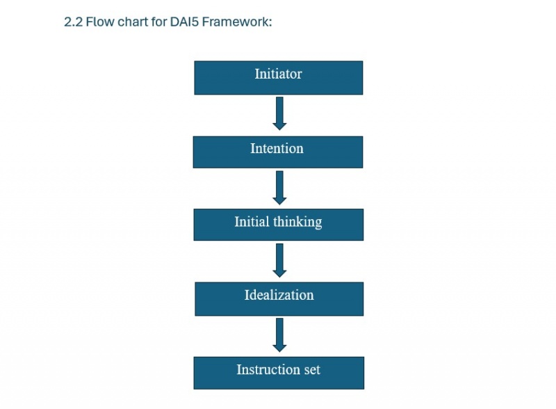
We followed this framework to find the good solution for the problem which is totally different from the conventional approaches, this approach more focused on subjective experience is about how each person perceives and interprets the world in their own unique way. It's based on individual feelings, thoughts, and personal experiences rather than objective facts. This framework consist of 5 Is which we followed to achive our objectives as;
2.1.1 Initiator:
In this study, the author play role of the initiator, anchoring this process through his philosophical insight: "I am My Consciousness" This concept underscores the intrinsic connection between personal identity and self-awareness, proposing that our consciousness and thoughts not only shape our actions but also influence how we perceive reality. By integrating this perspective, Dr. Indra introduces crucial philosophical, psychological, and ethical dimensions into the framework, which in turn fosters reflective thinking. By fostering an awareness of the soul, the author aligns the research process with a higher intent serving not only technical goals but also fulfilling a spiritual purpose. In this context, the Optimization of 2D Element Mesh in plane stress and its integration with the DAI5 framework reflect a conscious seeking of knowledge and truth, grounded in the remembrance of the Creator.
2.1.2 Intention:
In the context of the DAI5 framework, intention plays a pivotal role in defining the purpose and desired outcome of the thought process. This aligns with the philosophy of consciousness, where intentionality guides mental engagement with precision and focus. Throughout this study, having a clear understanding of the intention allowed us to maintain focus on the primary objective: conducting a 2D element plane stress analysis of a shell structure. The goal of this analysis was to determine the optimal combination of mesh methods and mesh sizes that would achieve the best accuracy, while maintaining constant structural parameters such as thickness, length, and boundary conditions. This clear intention shaped every step of the research, ensuring that each decision, from mesh generation to boundary condition application, was aligned with the objective of producing precise and reliable results within an efficient computational framework. By emphasizing intentional thinking, we were able to approach the problem methodically and with mindfulness, ensuring that each phase of the analysis was coherent with the broader aim of optimizing the mesh configuration. This clarity helped mitigate distractions, streamline the process, and foster a structured analysis focused on optimizing the 2D element mesh for the shell structure which will help the local community in term of energy reduction and time saving and hence the cost.
The deliberate focus on intention throughout the study not only ensured that the research remained aligned with its core objectives but also facilitated the development of an efficient analytical approach. By maintaining the structural parameters constant, we were able to isolate the impact of different mesh configurations and ultimately identify the combination that provided the optimal balance of accuracy and computational efficiency.
2.1.3 Initial Thinking:
The initial thinking phase of the DAI5 framework serves as an exploratory stage where ideas and information are gathered without the constraints of immediate judgment or decision-making. During this phase, participants are encouraged to brainstorm, reflect, and contemplate multiple facets of the problem at hand. The freedom to explore various ideas fosters a holistic approach, allowing intuition and past experiences to guide the generation of creative insights. The aim is to gather as much relevant information as possible before narrowing down to more focused solutions. While applying this concept to the 2D element stress analysis of a shell structure, the nature of the problem becomes the primary focus: the shell is subjected to specific boundary conditions and external uniform force, and the goal is to evaluate the resulting stress field. In particular, the problem centers on understanding how external forces and boundary constraints influence the structural integrity of the polycarbonate shell under static loading conditions. This involve the following;
1) Information Search:
At this stage, a 2D element analysis is being conducted on a cylindrical shell made of polycarbonate, a thermoplastic known for its toughness, impact resistance, and thermal stability. Polycarbonate is frequently chosen in engineering applications for its ability to withstand applied loads while maintaining structural integrity. This makes it a suitable material for pressure-bearing applications, such as cylindrical shells, where the structure must resist deformation under various loading conditions.The focus of this analysis is on the 2D element approach, which is especially effective for structures like cylindrical shells. This method simplifies computation while still delivering accurate results. By using 2D plane stress assumptions, the complexity of a full 3D analysis is reduced, concentrating only on the significant stress components within the shell’s plane. This approach is suitable when the shell's thickness is relatively small compared to its length and radius, as is the case here. Underlying principles for stress analysis are; Hooke’s Law provides the foundational relationship between stress and strain in elastic materials, while the stress equilibrium equations ensure that forces within a structure are balanced under static loading. Together, these principles are essential for accurately analyzing the behavior of materials and structures in engineering applications, particularly when using methods such as Finite Element Analysis (FEA). In the context of a cylindrical polycarbonate shell, understanding these principles is crucial for determining how the material will respond to applied forces and ensuring that it maintains structural integrity under load.
2) Nature of the Problem:
The focus of this analysis is on the behavior of a cylindrical shell under external uniform force, with the aim of understanding how the material responds under static loading conditions. The shell in question is made of polycarbonate, with mechanical properties that include a modulus of elasticity and Poisson's ratio specific to polycarbonate's behavior under loading conditions. Moreover, polycarbonate a versatile thermoplastic material widely used in engineering and industrial applications due to its mechanical properties such as high impact resistance, toughness, and thermal stability. These properties make polycarbonate an ideal choice for applications requiring structural integrity under various loads, including pressure vessels, piping systems, and storage tanks etc. In additon we are searching for the appropriate mesh configuration that balanced the accuracy and computational time.
3) Stress Analysis:
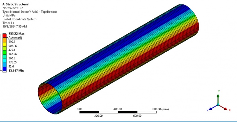
To evaluate the stress field within the shell using 2D element analysis. The primary focus is on understanding how the plane stress is distributed within the shell structure. Specifically, the goal is to assess how the polycarbonate material responds to the applied forces, considering both the radial force loading and the fixed boundary conditions. Normal Stress in the x and y directions; The analysis involves calculating the stresses acting on the material’s plane, which are critical for determining how the shell will deform under load. When a uniform radial force is applied, these stresses help identify regions of potential failure or deformation.
2.1.4 idealization:
Idealization involves envisioning the best possible scenarios and solutions while transcending present limitations. This stage encourages creative thinking and prompts individuals to consider solutions beyond the immediate constraints. In scientific and engineering analysis, idealization plays a critical role in simplifying complex problems by making certain assumptions that allow for more focused and efficient modeling, without losing sight of the ultimate goal of accuracy and precision. In this analysis, the assumptions reflect an idealization of the shell's behavior under given loading conditions are given by;
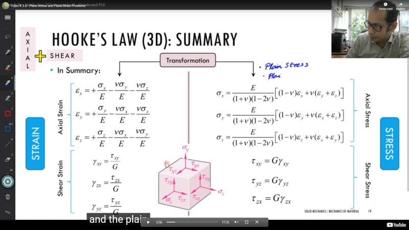
1) By assuming linear elastic behavior for the polycarbonate material, the analysis focuses on the portion of the material’s behavior that is predictable and consistent with Hooke's Law, while disregarding complexities such as plastic deformation or fracture. This assumption simplifies the problem, enabling the analysis to stay within the elastic regime where stress is proportional to strain[21]. By governing the stress-strain relationships with Hooke's Law, the analysis leverages the linear relationship between stress and strain in elastic materials, which is well understood and easily modeled. This idealization reflects a best-case scenario where the material behaves predictably within its elastic limit, allowing for precise calculation of stress and strain distributions without the need for more complex nonlinear models for 2d element analysis of shell. The required equations are[18, 19] as shown in the Hook’s law matrix equation;
2) The application of plane stress conditions is another idealization that allows the problem to be reduced from three dimensions to two, thus enhancing computational efficiency while maintaining accuracy for structures where the thickness is much smaller than the length and radius. This approach is not about ignoring the z-axis stress but recognizing that, for the purposes of this analysis, the deformation in the z-direction is negligible and will not significantly affect the in-plane stress and strain behavior. Similarly, excluding z-axis terms (σz=0, and τxz=τyz=0 in the following equations) from the governing equations aligns with the assumption of plane stress and emphasizes the in-plane behavior of the shell. This idealization ensures that the model remains efficient and tractable while still capturing the essential behavior of the shell under pressure loading.
Axial Stress for Transformation (Plane Stress):
Plane stress matrix equation[22]:
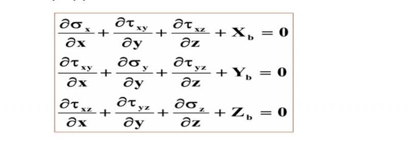
Stress equibrium equations by putting Xb=0, Yb=0, Zb=0, σz=0, τxz=0, and τyz=0 to get plane stress equation[22]:
3) By applying 2D plane stress assumptions, the need for a full 3D analysis is simplified, focusing primarily on the key stress components that occur within the plane of the shell. This approach reduces computational complexity while capturing the most relevant stress behavior.
4) The shell is made of polycarbonate becaause of exceptional applications in real world.
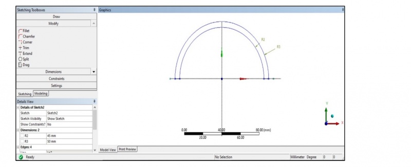
5) Dimensions:
Length: 500 mm
Outer radius: 50 mm
Inner radius: 45 mm
Wall thickness: 5 mm
The shell's geometry is representative of thin-walled cylindrical structures commonly found in engineering applications, where the ratio of the shell's thickness to its radius is small enough to justify the assumption of plane stress condition. The wall thickness of 5 mm, relative to the shell's overall dimensions, suggests that the shell's structural response will primarily involve in-plane stresses, with negligible out-of-plane deformations.
6) Boundary Conditions:
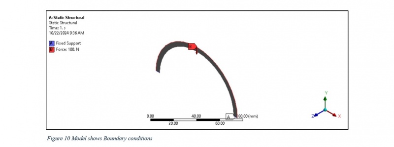
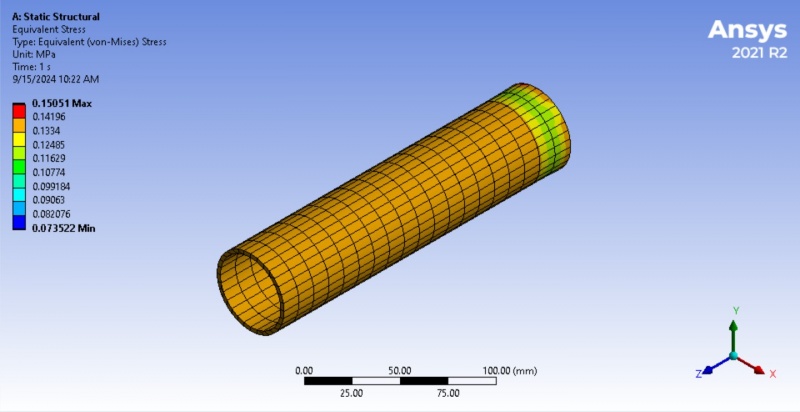
For this analysis, the following boundary conditions have been applied: Force: A uniform force of 100 N is applied in the negative y-direction. This force simulates real-world conditions where cylindrical shells, such as pressure vessels or pipes, are subjected to forces that deform the structure. Fixed Support: The shell is fixed at two edges, ensuring no displacement occurs at these points. This boundary condition restricts movement at the support locations and focuses the analysis on the stress response of the material elsewhere. These boundary conditions are appropriate for static structural problems, where the shell is subjected to continuous force loading. Understanding how these forces affect the stress field within the shell is crucial for ensuring the material’s structural integrity under load.
7) Constraints:
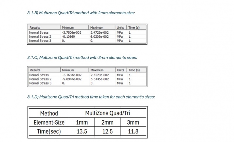
In this study, a reference value of 0.03 MPa was selected to calculate the error in normal stress in the x-direction, serving as the benchmark for evaluating accuracy across different mesh configurations. Additionally, a computational time constraint of 13.0 seconds was established to identify the minimum time required for each solution run, ensuring that the selected configurations meet both accuracy and efficiency criteria. These constraints provide a structured basis for assessing the performance of various mesh methods and element sizes under consistent conditions.
2.1.5 Instruction set:
The instruction set phase of the DAI5 framework bridges the gap between theoretical ideals and practical implementation. It involves translating abstract concepts and objectives into clear, actionable steps that can be carried out to achieve the desired outcomes. In engineering and computational analysis, this stage ensures that the ideas and assumptions made during the idealization phase are effectively operationalized through a systematic approach. In this analysis, a structured instruction set is developed to translate the idealized solutions and assumptions into concrete, actionable steps. The aim is to ensure that the methodology aligns with the theoretical framework established in the earlier phases while focusing on practical implementation using ANSYS 2021R2. The analysis involves a shell structure made from polycarbonate, a common thermoplastic known for its toughness and elasticity, under specific boundary conditions, while varying the mesh element size and method. The shell dimensions are kept constant, and we examine the effect of changing mesh configurations on the stress distribution within the shell.
2.1.5a Model Setup:
The initial phase of the analysis involved creating the geometric model of the shell using DesignModeler in ANSYS 2021R2. The geometry was modeled as a shell structure, reflecting a typical cross-section of pressure vessels or pipelines subjected to uniform force. The following dimensions were applied:
Length: 500 mm
Outer radius: 50 mm
Inner radius: 45 mm
Wall thickness: 5 mm
This shell structure model was selected due to its practical application in various industrial fields, where cylindrical shells are subjected to various loads from fluids or gases. Given the small thickness of the shell relative to its other dimensions, the model was simplified using 2D element analysis under plane stress condition. This assumption is valid since the deformation along the z-axis (out-of-plane) is negligible when the thickness is small in comparison to the shell’s length and radius.The shell geometry allows for efficient simulation of the stress distribution in the shell, while the 2D analysis approach simplifies the model without compromising on accuracy. The geometry was carefully defined to reflect real-world applications and to ensure that the results could be generalized to other pressure-bearing structures made from polycarbonate or similar materials.
2.1.5b Material Properties:
The material chosen for this analysis was polycarbonate, a well-known thermoplastic that exhibits excellent toughness and resilience, making it ideal for use in pressure-bearing structures such as pipelines, pressure vessels, and protective coverings. Polycarbonate is favored for its high impact resistance and ability to retain structural integrity under varying loading conditions. The following material properties were assigned in the ANSYS material library:
These material properties are critical in defining the linear elastic behavior of the polycarbonate shell, allowing the use of Hooke’s Law to model the stress-strain relationship within the material. By assuming linear elasticity, the analysis remains within the elastic regime of the material, focusing on the behavior of polycarbonate without considering plastic deformation or failure. This simplification streamlines the calculations while providing an accurate representation of the material’s response to internal pressure.
2.1.5c Meshing: (Varying the Mesh Element Size and Method)
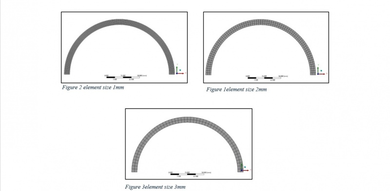
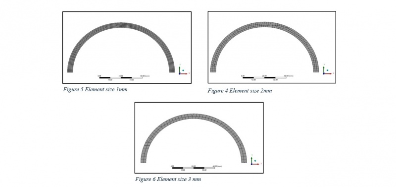
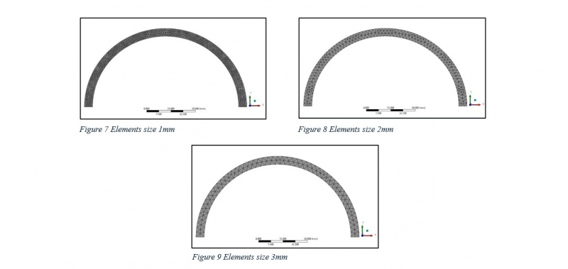
The key variable in this analysis was the mesh configuration, which was systematically varied to examine the impact of different mesh element sizes and meshing methods on the accuracy and computational efficiency of the results. The following meshing methods were tested in ANSYS:
Multizone Quad/Tri method: This method combines quadrilateral and triangular elements to generate a structured mesh that adapts well to the complex geometry of the cylindrical shell. The multizone approach provides a balance between element accuracy (quadrilateral elements) and flexibility (triangular elements).
Quadrilateral Dominant method: This method prioritizes the use of quadrilateral elements, which are known to provide higher accuracy for structural analysis. Quadrilateral elements are particularly effective at capturing stress and strain distributions in flat and curved regions of the shell.
Triangle method: A purely triangular element mesh was applied to evaluate the performance of this simpler meshing method. Triangular elements are commonly used in FEA due to their flexibility in conforming to complex geometries, but they tend to be less accurate than quadrilateral elements.
For each meshing method, the element size was varied as follows: 1 mm, 2 mm, and 3 mm. Smaller element sizes were expected to yield more accurate results by capturing finer details in the stress and strain distributions, particularly in areas with high stress concentrations. However, smaller element sizes increase the computational cost. Larger element sizes, on the other hand, reduce the computational time but may lead to a loss of accuracy in critical regions of the shell.By systematically testing these mesh sizes and methods, the goal was to identify the optimal combination that provided the best accuracy. This step is crucial for determining the most effective meshing strategy for future simulations of similar structures.
A) Multizone Quad/Tri method with varying elements sizes:
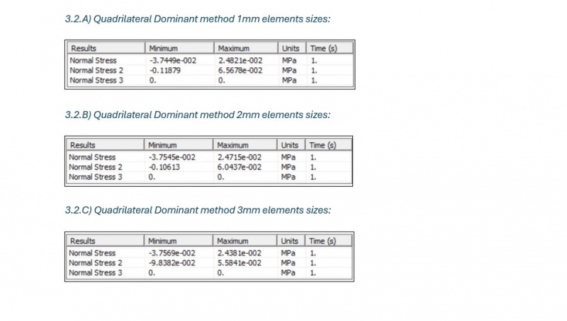
B) Quadrilateral Dominant method with varying elements sizes:
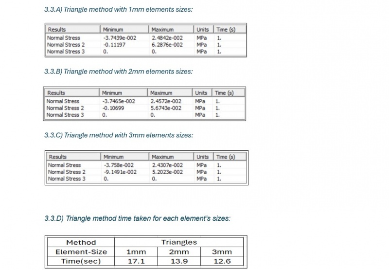
C) Triangle method with varying elements sizes:
2.1.5d Boundary Conditions:
To simulate real-world loading scenarios, the following boundary conditions were applied to the polycarbonate shell: Fixed Support: The shell was fixed at both ends along the axial direction (x-direction). This boundary condition ensured that no displacement occurred in the axial direction, simulating a scenario where the ends of the shell are constrained or anchored, as in pressure vessels or pipes supported at both ends.
External force: A constant external force of 100 N was applied uniformly to the the shell. This force simulated typical internal loading conditions experienced by cylindrical shells in real-world applications. These boundary conditions were designed to simulate the most realistic loading conditions for the polycarbonate shell, allowing for accurate analysis of the shell’s response to external force.
2.1.5e Solver and Stress-Strain Analysis:
With the geometry, material properties, mesh configurations, and boundary conditions defined, the static structural solver in ANSYS was used to compute the stress distribution across the shell. The solver focused on the following key aspects of the shell’s behavior:
Normal Stress in the x and y directions: These stresses represent the force per unit area acting perpendicular to the material’s surface. Normal stresses are crucial for understanding how the shell deforms under radial force and provide insights into potential regions of failure, particularly near the fixed supports
2.2 Flow chart for DAI5 Framework:
2.2 Flow chart for FEM Using Ansys:
3. Results and discussion
The following are the results of the 2D elements plane stress analysis of shell structure;
From the results it has been deducted;
1. Stress analysis:
1.a Multizone Quad/Tri Method:
At a 1 mm element size, the maximum normal stress in the x-direction recorded was 0.0248 MPa, with a minimum stress of -0.0374 MPa respectively, and the total computational time was 13.5 seconds. The high-resolution mesh with smaller element sizes accurately captures stress variations, especially around stress concentration zones. However, this accuracy comes at the cost of longer computational time. The 1 mm mesh size, while providing precise stress values, requires a significant time investment due to the increased number of elements and corresponding calculations. With an increase to a 2 mm element size, the maximum normal stress in x-direction decreased slightly to 0.0247 MPa, while the minimum stress reduced to -0.0375 MPa. The computational time also decreased to 12.5 seconds. This indicates that a moderate increase in element size results in a slight reduction in stress resolution, though the decrease in stress concentration is not substantial. The drop in computational time reflects the decreased number of elements, which leads to faster calculations while maintaining acceptable accuracy. For the 3 mm element size, the maximum normal stress in x-direction was further reduced to 0.0245 MPa, and the minimum stress reached -0.0376 MPa, with a computational time of 11.8 seconds. The trend of reduced stress values with larger element sizes is evident, with the coarser mesh having a smoothing effect on stress variations. Although the computation is faster with the larger elements, there is a corresponding reduction in the resolution of localized stress concentrations. The results from the Multizone Quad/Tri Method show that smaller element sizes (1 mm) provide detailed stress analysis but require longer computational time. As the element size increases, there is a trade-off: computational time decreases, but stress accuracy is compromised. For applications where precision is critical, the 1 mm element size is recommended, while for faster computations with acceptable accuracy, 2 mm or 3 mm element sizes offer a good balance.
1.b Quadrilateral Dominant Method:
At a 1 mm element size, the maximum normal stress in x-direction was 0.0248 MPa, with a minimum stress of -0.0374 MPa, and the total computational time was 14.2 seconds. The Quadrilateral Dominant Method performs similarly to the Multizone Quad/Tri Method at this mesh resolution, capturing stress variations in the structure effectively, albeit with slightly higher computation times due to the method's focus on quadrilateral element shapes. For the 2 mm element size, the maximum normal stress in x-direction decreased to 0.02471 MPa, and the minimum stress remained stable at -0.0375 MPa, while the computational time decreased to 13.7 seconds. The reduction in time is significant, but the stress results remain highly accurate. This shows that the Quadrilateral Dominant Method is relatively stable in terms of stress accuracy as the mesh becomes coarser, making it suitable for analyses where moderate stress accuracy is acceptable. At the 3 mm element size, the maximum normal stress in x-direction dropped to 0.0243 MPa, with a minimum stress of -0.0376 MPa, and the computational time decreased to 12.6 seconds. The reduction in stress accuracy is minimal, though larger element sizes mean a loss of resolution in stress concentrations. However, this method remains efficient for structural analysis with larger mesh sizes, where precision in stress concentration regions is not the primary concern. The Quadrilateral Dominant Method shows robustness across different element sizes, with only minimal changes in stress values as the mesh becomes coarser. The computational time is slightly higher than the Multizone method, but the method is consistent in maintaining stress accuracy. This method is particularly advantageous for general structural analysis where both time efficiency and moderate stress resolution are required.
1.c Triangle Method:
For the 1 mm element size, the maximum normal stress in x-direction recorded was 0.02484 MPa, with a minimum stress of -0.0374 MPa, and the computational time was 17.1 seconds. The Triangle Method is the most computationally expensive, but it yields slightly higher stress values than the other methods. The triangular elements offer flexibility in capturing geometric details, resulting in better stress concentration capture. However, the increased computation time reflects the complexity of using triangular elements for stress analysis. At the 2 mm element size, the maximum normal stress in x-direction decreased to 0.0246 MPa, and the minimum stress remained at -0.0375 MPa, with the computational time reduced to 13.9 seconds. The decrease in computational time is substantial, yet the method maintains accurate stress analysis, particularly in regions with complex stress distributions. This balance between accuracy and efficiency makes the Triangle Method suitable for detailed structural analyses where stress concentrations are critical. For the 3 mm element size, the maximum normal stress in x-direction was further reduced to 0.0243 MPa, and the minimum stress was -0.0376 MPa, with a computational time of 12.6 seconds. Similar to the other methods, the larger element size results in faster computations but less accurate stress concentration analysis. However, the Triangle Method continues to provide higher stress values compared to the other methods, even at larger element sizes, due to its ability to adapt to complex geometries. The Triangle Method provides the most detailed stress analysis at finer mesh sizes (1 mm), but this comes at a significantly higher computational cost. As the element size increases, the method becomes more computationally efficient, though it remains slower than the other methods. The Triangle Method is particularly useful for applications where capturing detailed stress distributions in geometrically complex regions is critical, despite the higher computational time. For less critical stress analyses, larger element sizes (2 mm or 3 mm) offer a good compromise between time and accuracy.
4. Optimization of mesh configuration:
Based on the table analysis in excel as shown in (Figure 11), we set a constraint of 0.03 MPa for normal stress in the x-direction and calculated the absolute errors for each mesh configuration, which comprised various mesh methods and element sizes. Our objective was to identify the mesh configuration yielding the lowest absolute error in normal stress in the x-direction while meeting the specified time constraint. Additionally, we selected a time constraint of 13.0 seconds and classified each configuration's computational time as either "MIN" or "MAX" relative to this threshold. Following the time constraint evaluation, we identified four configurations marked as “MIN” (with times of 12.5 seconds, 11.8 seconds, 12.6 seconds, and 12.6 seconds). Among these configurations, we further investigated to determine the one with the lowest absolute error in normal stress in the x-direction. Our analysis revealed that the configuration with a time of 12.5 seconds also corresponded to the smallest absolute error in the x-direction, recorded at 17.6. Consequently, we selected the optimal mesh configuration, which consisted of the "MultiZone Quad/Tri" mesh method with a 2 mm element size. This configuration provided a normal stress in the x-direction of 0.02472 MPa and achieved the minimum computational time of 12.5 seconds, thus meeting both accuracy and efficiency objectives.
5. Conclusion
This study demonstrates the effectiveness of different meshing techniques for 2D element stress analysis in polycarbonate shell structures under static loading. By applying the DAI5 conscious thinking framework, we systematically evaluated the performance of three mesh methods Multizone Quad/Tri, Quadrilateral Dominant, and Triangle at varying element sizes. Key findings include: 1) Multizone Quad/Tri Method: Provides the best balance of accuracy and computational efficiency at 2 mm element size, capturing stress concentration zones effectively while minimizing computational time. 2) Quadrilateral Dominant Method: Offers consistent stress accuracy across different mesh sizes but requires slightly longer computational times than the Multizone method. This method is optimal for general structural analysis where moderate stress resolution is acceptable. 3) Triangle Method: Though more computationally expensive, this method provides superior accuracy in capturing stress distributions in geometrically complex regions, making it ideal for detailed structural analyses despite longer computation times. The study highlights that smaller element sizes yield more accurate results but at the expense of increased computational time. For practical engineering applications, selecting the optimal mesh configuration depends on the specific trade-offs between precision and efficiency. The DAI5 framework facilitated a reflective and intentional approach to optimizing mesh configurations, ensuring that the analysis remained focused on both technical accuracy and ethical considerations.
References
[1] L. Xie, "Research on finite element static analysis in mechanical vehicle structure design," in Applied Mechanics and Materials, 2014, vol. 511-512, pp. 606-610, doi: 10.4028/www.scientific.net/AMM.511-512.606. [Online]. Available: https://www.scopus.com/inward/record.uri?eid=2-s2.0-84896869706&doi=10.4028%2fwww.scientific.net%2fAMM.511-512.606&partnerID=40&md5=bf6a3024c308427fce030cffdc70e32d
[2] C. M. Wai, A. Rivai, and O. Bapokutty, "Modelling optimization involving different types of elements in finite element analysis," in IOP Conference Series: Materials Science and Engineering, 2013, vol. 50, 1 ed., doi: 10.1088/1757-899X/50/1/012036. [Online]. Available: https://www.scopus.com/inward/record.uri?eid=2-s2.0-84893574266&doi=10.1088%2f1757-899X%2f50%2f1%2f012036&partnerID=40&md5=f1f018e49b16a62d4e13fc279deb1527
[3] P. Mihaylova, N. Baldanzini, and M. Pierini, "Considerations on 1D beam concept modelling for the vehicle structure," in International Conference on Noise and Vibration Engineering 2012, ISMA 2012, including USD 2012: International Conference on Uncertainty in Structure Dynamics, 2012, vol. 5, pp. 3793-3808. [Online]. Available: https://www.scopus.com/inward/record.uri?eid=2-s2.0-84906330927&partnerID=40&md5=14669964066ea29b3d1fdf60b455df5b. [Online]. Available: https://www.scopus.com/inward/record.uri?eid=2-s2.0-84906330927&partnerID=40&md5=14669964066ea29b3d1fdf60b455df5b
[4] A. J. M. Ferreira and N. Fantuzzi, "Plane stress," in Solid Mechanics and its Applications, vol. 157, 2020, pp. 171-205.
[5] J. E. Akin, "Enhanced moment and shear recovery for classic beams and frames," Engineering Structures, Article vol. 174, pp. 814-825, 2018, doi: 10.1016/j.engstruct.2018.07.068.
[6] D. Ambrosini, R. H. Codina, O. Curadelli, and C. A. Martínez, "Structural analysis of the CAREM-25 nuclear power plant subjected to the design basis accident and seismic loads," Annals of Nuclear Energy, Article vol. 108, pp. 42-56, 2017, doi: 10.1016/j.anucene.2017.04.029.
[7] A. Setiawan, R. L. Vollum, L. Macorini, and B. A. Izzuddin, "Numerical modelling of punching shear failure of reinforced concrete flat slabs with shear reinforcement," Magazine of Concrete Research, Article vol. 73, no. 23, pp. 1205-1224, 2021, doi: 10.1680/jmacr.19.00562.
[8] Q. Liu, D. Li, and J. Tan, "Rating the Crack-Resistance effect for a Steel Truss Bridge Based on 3D Fracture Mechanics Model," in IOP Conference Series: Earth and Environmental Science, 2020, vol. 510, 5 ed., doi: 10.1088/1755-1315/510/5/052088. [Online]. Available: https://www.scopus.com/inward/record.uri?eid=2-s2.0-85089398594&doi=10.1088%2f1755-1315%2f510%2f5%2f052088&partnerID=40&md5=8946549d18e714a512aec7afa7065cea
[9] CRAYON, "Everything you need to know about Polycarbonate sheets." [Online]. Available: https://www.crayonroofings.com/blog/everything-you-need-to-know-about-polycarbonate-sheets/.
[10] P. Diekmann and M. Horländer, "Transparent safety: Polycarbonate protective glazing for roofs, walls and machines," ThyssenKrupp techforum, Review no. DEC., pp. 80-85, 2004. [Online]. Available: https://www.scopus.com/inward/record.uri?eid=2-s2.0-14544283326&partnerID=40&md5=1b561a2959b3c76ad64cb7757fc77d40.
[11] G. L. Garcez, R. Picelli, and R. Pavanello, "Bi-directional evolutionary topology optimization based on stress minimization under design-dependent surface loads," Engineering Optimization, Article vol. 55, no. 7, pp. 1168-1188, 2023, doi: 10.1080/0305215X.2022.2065481.
[12] K. Nabaki, J. Shen, and X. Huang, "Stress Minimization of Structures Based on Bidirectional Evolutionary Procedure," Journal of Structural Engineering (United States), Article vol. 145, no. 2, 2019, Art no. 04018256, doi: 10.1061/(ASCE)ST.1943-541X.0002264.
[13] H. Svärd, "Interior value extrapolation: a new method for stress evaluation during topology optimization," Structural and Multidisciplinary Optimization, Article vol. 51, no. 3, pp. 613-629, 2015, doi: 10.1007/s00158-014-1171-2.
[14] X. Peng and Y. Sui, "Method of first-order approximations of inter force for structural topology optimization with stress constraints," Jixie Qiangdu/Journal of Mechanical Strength, Article vol. 38, no. 5, pp. 990-995, 2016, doi: 10.16579/j.issn.1001.9669.2016.05.016.
[15] D. A. Indra, "DAI5 Framework," 2024. [Online]. Available: https://air.eng.ui.ac.id/index.php?title=Main_Page.
[16] T. abbey, "Plane Stress and Plane Strain – simplifying models," 2019. [Online]. Available: https://fetraining.net/plane-stress-plane-strain/?form=MG0AV3.
[17] G. Quaranta, M. Ziane, E. Haug, J. L. Duval, and F. Chinesta, "A minimally-intrusive fully 3D separated plate formulation in computational structural mechanics," Advanced Modeling and Simulation in Engineering Sciences, Article vol. 6, no. 1, 2019, Art no. 11, doi: 10.1186/s40323-019-0135-x.
[18] J. Górski and W. Pietraszkiewicz, "The 10th Jubillee Conference "Shell Structures: Theory and Applications", SSTA2013, Oct. 16-18, 2013, Gdańsk (Poland)," in Archives of Civil Engineering, 2013, vol. 59, 4 ed., pp. 579-581, doi: 10.2478/ace-2013-0032. [Online]. Available: https://www.scopus.com/inward/record.uri?eid=2-s2.0-84893353031&doi=10.2478%2face-2013-0032&partnerID=40&md5=3170c0618347d43ca3b35521d0cb52f8
[19] D. Chapelle, "Some new results and current challenges in the finite element analysis of shells," in Differential Geometry: Theory And Applications, 2008, pp. 185-221.
[20] G. Quaranta, M. Ziane, F. Daim, E. Abisset-Chavanne, J. L. Duval, and F. Chinesta, "On the coupling of local 3D solutions and global 2D shell theory in structural mechanics," Advanced Modeling and Simulation in Engineering Sciences, Article vol. 6, no. 1, 2019, Art no. 1, doi: 10.1186/s40323-019-0125-z.
[21] J. M. Gere and B. J. Goodno, Mechanics of Materials. Cengage Learning, 2012.
[22] "Review of Elasticity Equations." [Online]. Available: https://imechanica.org/files/PlaneElements.pdf.
End of Mid_Term_
DAI5 Framework:
Hello, I am Tanveer Khan presenting the DAI5 Framework, an innovative approach developed by Dr. Ahmed Indra (DAI). This method, DAI5, focuses on intentions, initial thinking, idealizations, and instruction sets for effective problem-solving. I discuss the unique aspects of DAI5 and how it differs from traditional approaches, emphasizing the importance of clarity and specificity in instructions. Viewers are encouraged to understand the significance of setting clear objectives and simplifying complex problems.
Total deformation analysis of a bar using 1D elements and Ansys 2021R2:
2D plane stress analysis using Ansys 2021R2:
Pipe stress analysis using Ansys 2021R2:
I used the following specifications for the stress analysis of the pipe using the Ansys 2021R2;
Material:
1)Structural steel.
Geometric dimensions:
1) Length: 200mm.
2) Outer Diameter: 50mm.
3) Inner Diameter: 45mm.
4) Thickness: 2.5mm.
Boundary conditions:
1) Fixed right end.
2) Applied load to the left end (Load= 50N).
<<<Total deformation:>>>
The image shows a structural analysis result from ANSYS software. The analysis focused on the total deformation of a pipe under 50 N load. The color gradient ranges from red (maximum deformation) to blue (minimum deformation). Red represents the area with the highest deformation, around 0.00013372 mm. Blue indicates the region with little or no deformation. Based on the image, the highest deformation occurs at the left end of the pipe, which is colored red, while the least deformation occurs at the opposite end, in blue which is 0 mm.
<<<Strain:>>>
The image shows strain analysis results from an Ansys simulation, specifically for a pipe, analyzed using static structural analysis. The result shows the elastic strain distribution in a pipe under 50N load. The maximum strain occurs near the right end of the pipe, possibly due to concentrated stresses, while the rest of the pipe experiences a more uniform, lower strain. The color scale on the left ranges from blue (minimum strain value 3.7099×10^−7) to red (maximum strain value 7.573×10^−7).
Blue/Cyan/Green: These colors represent regions experiencing low to moderate elastic strain.
Yellow/Orange/Red: These regions experience higher elastic strain, with red indicating the maximum strain values.
The highest elastic strain (indicated by red and orange) is located toward the right end of the pipe. This suggests that this portion is undergoing the most deformation under the applied load. On the other hand, the lowest strain (blue) is spread along the middle to the left side of the pipe. This indicates that these areas are relatively less affected by the applied loads, experiencing lower deformation.
<<<Stress:>>>
The given image shows the result of a finite element analysis (FEA) of a pipe under static structural loading 50N, likely performed in Ansys 2021 R2. The analysis focuses on the Equivalent Stress, specifically the von Mises stress, which is used to predict the yielding of materials under complex loading conditions. The color bar on the left indicates the magnitude of von Mises stress in MPa (megapascals), ranging from 0.073522 MPa (blue) to 0.15051 MPa (red). The color distribution on the pipe shows the areas experiencing different stress levels. Red and yellow areas near the end of the pipe are experiencing the highest stress, while blue and green areas are under lower stress. The highest stress 0.15051 MPa occurs near the end of the pipe, where the colors transition from green to yellow and red. The rest of the pipe has lower stress values, predominantly in the orange-yellow range, indicating that most of the structure is experiencing moderate stress levels. Blue areas, especially on the opposite end, indicate the regions under minimal stress.
Basic questions:
Question(1): Is the force term internal or external in stress-force relation? >>(Sigma= F/A)?
Question(2): Does stress force direction dependent?
Question(3): How do we form the global stiffness matrix based on element-wise stiffness matrices?
2D_beam stress_strain analysis using Ansys 2021R2:
Specifications in (millimeter):
1) Lenght = 4000mm.
2) Wall thickness= 3.4036mm
3) Width= 152.4mm.
Material:
Stainless steel.
Boundary conditions:
1) Simple supported on two ends.
2) Second-end applied Load= 4000N (UDL on 10mm patch in -y direction).
----2D-Stress:----
<<<Total deformation:>>>
The given image static structural analysis shows the total deformation of the structure, with a maximum displacement of 12.466 mm in the center (red) and a minimum of 0.003947 mm near the edges (blue). The color gradient from blue to red indicates how the deformation varies, with the highest strain occurring in the middle of the structure, suggesting significant bending or displacement under the applied load. The analysis highlights that the central section is most affected, while the edges experience minimal deformation, reflecting the load distribution across the structure.
<<<Equivalent Stress:>>>
The image shows the results of an equivalent (von Mises) stress analysis for the structure, with the stresses measured in megapascals (MPa). The maximum stress occurs at 300.52 MPa (red), and the minimum stress is 1.0292 MPa (blue). The stress distribution across the structure is represented by a color scale from blue (low stress) to red (high stress), indicating that the areas near the middle of the structure experience the highest stress, particularly in the region with yellow, orange, and red colors. The outer edges, shown in blue, experience the least stress. This type of analysis helps in identifying the most critical areas in the structure that are likely to fail under load. High-stress areas, such as the center, may require design or material changes to avoid failure.
<<<Nomral Stress:>>>
The image presents the results of a normal stress analysis along the X-axis, with stress measured in megapascals (MPa). The maximum normal stress is 152.81 MPa (red), and the minimum is -246.11 MPa (blue). The color gradient, ranging from blue to red, indicates regions of compressive (negative) and tensile (positive) stress, with compressive stress shown in shades of blue and tensile stress in shades of yellow to red. The central area of the structure experiences the most compressive stress (deep blue), while the outer edges near the middle are under the highest tensile stress (red). This distribution suggests that the structure is bending, with tensile stress on the convex side and compressive stress on the concave side, typical for a beam under bending loads.
----2D_Strain:----
<<<Equivalent Elastic Strain:>>>
The image shows the results of an equivalent elastic strain analysis, measured in units of strain (mm/mm). The maximum strain occurs at 0.0067731 (red), while the minimum strain is 3.1269e-5 (blue). The strain distribution follows a similar pattern to the previous analyses, with the highest strain concentrated in the middle portion of the structure (indicated by red and yellow), suggesting this area experiences the most deformation under load. The edges show significantly lower strain (blue areas), indicating less elastic deformation. The color gradient from blue to red shows how strain is distributed across the structure, with the highest strain concentrated in regions of maximum bending. This analysis helps to assess how much the material stretches or compresses elastically, ensuring that the structure remains within its elastic limit to avoid permanent deformation.
<<<Normal Elastic Strain:>>>
This image displays the results of a normal elastic strain analysis along the X-axis, measured in mm/mm. The maximum normal strain is 0.0025374 (red), and the minimum is -0.0053577 (blue). The distribution of strain is indicated by a color scale, where red to yellow represents tensile strain, and blue to green represents compressive strain. The central region of the structure, particularly in the lower section, shows the highest tensile strain (red and yellow), while the top of the structure exhibits significant compressive strain (blue). This distribution is consistent with the bending behavior of the structure, where tensile strain is concentrated on the convex side and compressive strain on the concave side. The strain values help evaluate the material's elastic behavior and how much deformation the structure undergoes under the applied loads.
shell plain stress_strain analysis using Ansys 2021R2:
<<<Using DAI5 Framework:>>>
<<<Initiator:>>>
The framework is founded and inspired by Prof. Dr. Ahmad Indra.
<<<Intention:>>>
The purpose of this analysis is to study the plain stress and plain strain conditions in a stainless steel cylindrical shell, using a 2D element analysis in ANSYS to examine the stress and strain distribution due to the applied pressure. The objective is to interpret and analyze the following:
1) Normal stress in the x and y directions.
2) Normal elastic strain in the x and y directions.
<<<Initial Thinking about the Problem:>>>
Information Search: I am conducting a 2D element analysis on the shell, which is appropriate for cases involving pressure loading on cylindrical shells.
Nature of the Problem: We are dealing with a static structural problem. The shell is subject to internal pressure, and our interest lies in understanding how this pressure affects the stress and strain fields inside the shell.
Model Specifications:
Length: 2000 mm
Outer radius: 80 mm
Inner radius: 75 mm
Wall thickness: 10 mm
Material Properties: The shell is made of stainless steel, a common choice for high-strength structural applications.
Boundary Conditions:
Pressure: 50 MPa applied on the mid-plane of the shell (acting radially_outward).
Displacement: Free in the x and y directions, fixed in the z-direction.
Support: Cylindrical support allowing radial displacement to be free, but axial and tangential directions are fixed.
<<<Idealization:>>>
Assumptions:
1) The analysis assumes the linear elastic behavior of the material.
2) 2D plain strain conditions are assumed, as the thickness of the shell is relatively small compared to its length.
3) The temperature is the ambient.
4) Underlying Laws and formulas excluding the z-axis terms from all to get the plain strain-stress as shown in the given picture.
5) Stress-Strain Relationships: Governed by Hooke's law for elastic materials excluding the z_axis terms.
6) Equilibrium Equations: Static equilibrium condition which ensures the structure remains stable under loading.
<<<Instruction Set:>>>
The analysis was conducted in ANSYS 2021R2 using the following procedure:
Model Setup: The geometry of the shell was created using a DesignModeler.
Material Properties: Stainless steel was assigned with appropriate elastic properties.
Meshing: A mesh was generated for the shell to accurately capture the stress and strain distribution by using an element size of 20mm and the Multizone Quad/Tri method.
Boundary Conditions: Radial displacement was allowed, and axial/tangential displacements were fixed as specified. A pressure of 50 MPa was applied.
Solver: Static analysis was performed to compute the stress and strain fields.
Interpretation of Post-Processing Results:
<<<Normal Stress in the x-direction (Sigma_x):>>>
Observation: The normal stress in the x-direction shows a consistent distribution across the shell, with regions of high stress in the center and gradually reducing toward the ends.
Interpretation: The stress in the x-direction is uniform due to the applied boundary conditions and pressure. This stress represents the axial load distributed across the length of the cylindrical shell, peaking at the center where the pressure is concentrated.
Max Stress: The maximum axial stress is 755.22 MPa.
Min Stress: The minimum axial stress is 13.147 MPa at the ends, which is typical near the constrained boundaries.
<<<Normal Stress in the y-direction (Sigma_y):>>>
Observation: The normal stress in the y-direction also shows a high concentration in the middle, with a gradient decreasing toward the shell's edges.
Interpretation: The circumferential stress arises from the internal pressure applied to the cylindrical shell. The distribution indicates the stress is concentrated in the central region where the load is applied, which is consistent with the pressure application and boundary constraints.
Max Stress: 755.22 MPa, occurring at the mid-plane.
Min Stress: 13.147 MPa, similar to the axial stress behavior near the boundaries.
<<<Normal Elastic Strain in the x-direction (E_x):>>>
Observation: The strain in the x-direction is proportional to the stress distribution, with the highest values appearing near the center and gradually reducing toward the ends.
Interpretation: The axial strain corresponds to the applied stress in the x-direction. The results show higher strain in the middle region of the shell, where the pressure-induced stress is highest. The strain decreases as we move toward the ends of the shell.
Max Strain: 0.0035093 mm/mm showing that the shell experiences significant elastic deformation in response to the applied pressure.
Min Strain: -0.0015275 mm/mm indicating slight compressive strain at the extremities.
<<<Normal Elastic Strain in the y-direction (E_y):>>>
Observation: The strain in the y-direction shows a similar distribution to the x-direction strain, with higher values in the center and lower values toward the boundaries.
Interpretation: This strain corresponds to the circumferential strain due to the applied pressure. The elastic deformation follows the stress distribution closely, indicating the shell's expansion under load.
Max Strain: 0.0035093 mm/mm indicating the shell experiences elastic deformation in the circumferential direction.
Min Strain: -0.0015275 mm/mm representing slight compressive behavior at the shell's ends.
Finite element equations from a 1D Partial Differential Equation (PDE) using the weighted residual method:
I will take the example of a simple 1D PDE for steady-state heat conduction without internal sources.
Algorithm, Flow chart, and python code for a 1D FEM:
1) Algorithm:
1) Input the parameters:
>Domain length (L)
>Number of elements (n)
>Thermal conductivity (k)
>(alpha) Coefficient of thermal expansion (1/°C)
>(E) Young's modulus in Pascals
>Boundary conditions at x=0 (Dirichlet) and x=L (Neumann)
2) Discretize the domain:
>Divide L into n elements, each of length h= L/n.
>Define nodes at points x(i)=i.h, for i=0,1,...,n.
3) Construct the element stiffness matrix:
>For each element, calculate the local stiffness matrix K(e)= k/h[[1 -1],[-1 1]]
4) Assemble the global stiffness matrix K:
>Initialize an (n+1)X(n+1) matrix K.
>Add each K(e) to the global matrix K at the appropriate node positions.
5) Apply boundary conditions:
>For Dirichlet (fixed value), set the first row/column in K and F to apply the temperature value.
>For Neumann (flux), modify the last row of F to include the flux value q at x=L.
6) Solve for nodal temperatures u:
>Solve the linear system K⋅u=F to get u (nodal temperatures).
7) Solve for Thermal strain:
>Solve the linear system Thermal strain = alpha * (u - T_ref) to get Thermal Strain (nodal)
8) Solve for Thermal stress:
>Solve the linear system Thermal stress = E * (Thermal Strain) to get Thermal stress (nodal)
9) display the results:
>Nodal Temperatures
>Thermal Stress at each node (in Pascals)
2) Flow Chart:
3) Python code:
1D Thermal analysis using web based Java script:
1) Javascript:
2) Gradient-style bar chart:
The 33 DAI5 Implementation Evaluation Criteria
I. Deep Awareness (of) I (DAI)
1. Consciousness of Purpose: Reflects understanding of the Creator's role in shaping the case study context.
2. Self-awareness: Demonstrates awareness of personal biases, assumptions, and roles in the analysis.
3. Ethical Considerations: Includes moral and ethical implications in addressing the case study.
4. Integration of CCIT (Cara Cerdas Ingat Tuhan): Maintains remembrance of The Creator throughout the essay.
5. Critical Reflection: Shows depth in connecting technical solutions to broader spiritual and societal impacts.
6. Continuum of Awareness: Evidence of uninterrupted and progressive conscious analysis.
II. Intention
7. Clarity of Intent: States a clear and purposeful intention aligned with the ultimate goal of the Creator’s recognition.
8. Alignment of Objectives: Aligns case study objectives with higher values and universal principles.
9. Relevance of Intent: Ensures the intention addresses real-world engineering needs effectively.
10. Sustainability Focus: Intends solutions that consider long-term environmental, societal, and economic impacts.
11. Focus on Quality: Demonstrates a conscious intention to prioritize reliability, accuracy, and precision.
III. Initial Thinking (about the Problem)
12. Problem Understanding: Clearly identifies and describes the engineering problem.
13. Stakeholder Awareness: Considers perspectives of all stakeholders impacted by the problem or solution.
14. Contextual Analysis: Places the problem within a relevant physical, social, and technical context.
15. Root Cause Analysis: Identifies underlying causes, not just symptoms of the problem.
16. Relevance of Analysis: Ensures the problem-solving process is grounded in practical and applicable insights.
17. Use of Data and Evidence: Employs credible, accurate, and sufficient data to support problem understanding.
IV. Idealization
18. Assumption Clarity: States all assumptions explicitly and justifies their relevance.
19. Creativity and Innovation: Proposes unique or unconventional idealized solutions while adhering to realism.
20. Physical Realism: Ensures the idealization adheres to physical laws and engineering principles.
21. Alignment with Intent: Ensures idealization aligns with the initial intention and overarching goals.
22. Scalability and Adaptability: Considers whether the idealized solution is scalable and adaptable to different contexts.
23. Simplicity and Elegance: Proposes solutions that are efficient, simple, and elegant while solving complex problems.
V. Instruction (Set)
24. Clarity of Steps: Outlines each step of the solution process clearly and logically.
25. Comprehensiveness: Includes all relevant aspects of the solution, leaving no gaps.
26. Physical Interpretation: Explains the physical meaning of all numerical results or design decisions.
27. Error Minimization: Includes procedures to reduce errors in solution implementation.
28. Verification and Validation: Provides methods for verifying and validating the solution.
29. Iterative Approach: Demonstrates readiness to iterate and refine the solution if needed.
30. Sustainability Integration: Considers sustainable practices within the solution execution.
31. Communication Effectiveness: Presents instructions in a way that is understandable and actionable by others.
32. Alignment with the DAI5 Framework: Maintains coherence with all preceding DAI5 steps.
33. Documentation Quality: Provides clear, complete, and professional documentation of the solution.


