Difference between revisions of "Benarido Amri"
(→Static 2 Dimensional Simulation of a Single Blade) |
(→Energy Conversion System) |
||
| Line 257: | Line 257: | ||
The increase in velocity in area 4 can be explained simply as the fluids way of maintaining the same flow rate throughout the control volume. The equation is Q1 = Q2 or V1 * A1 = V2 * A2, because of the obstruction caused by the blade, the area of the control volume decreases, thus to maintain the same output flowrate, the velocity of the air must increase as well. Creating the shape and pattern as seen in the figure above. | The increase in velocity in area 4 can be explained simply as the fluids way of maintaining the same flow rate throughout the control volume. The equation is Q1 = Q2 or V1 * A1 = V2 * A2, because of the obstruction caused by the blade, the area of the control volume decreases, thus to maintain the same output flowrate, the velocity of the air must increase as well. Creating the shape and pattern as seen in the figure above. | ||
| + | |||
| + | == Revised Static 2-Dimensional Single Blade Simulation == | ||
| + | |||
| + | === Parameters === | ||
| + | |||
| + | *Box geometry properties: 0.1 m X 0.3 m X 1 m | ||
| + | *Base mesh: 10 m X 10 m X 0.1 m at 200 X 200 X 1 division | ||
| + | *Velocity reference value: 0.01 m/s | ||
| + | *Simulation mode: Steady-state, laminar, incompressible | ||
| + | *Initial condition = Fixed value velocity with 0 m/s speed | ||
| + | |||
| + | === Result === | ||
| + | |||
| + | ==== Pressure ==== | ||
| + | |||
| + | [[File:Pressure_00.png]] | ||
| + | |||
| + | ==== Velocity ==== | ||
| + | |||
| + | [[File:Velocity_000.png]] | ||
| + | |||
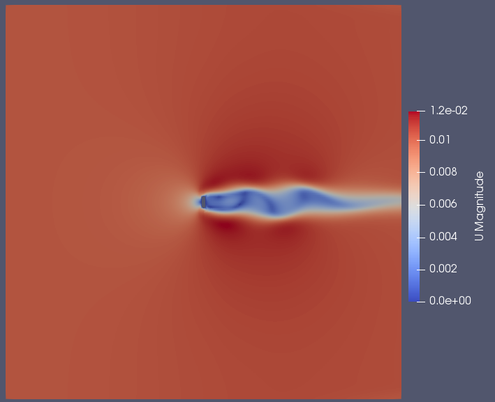
| + | Due to the much larger ratio between the control volume and blade size, a clear freestream region is visible outside of a certain radius of the blade. | ||
| + | |||
| + | [[File:Velocity_0000.png]] | ||
| + | |||
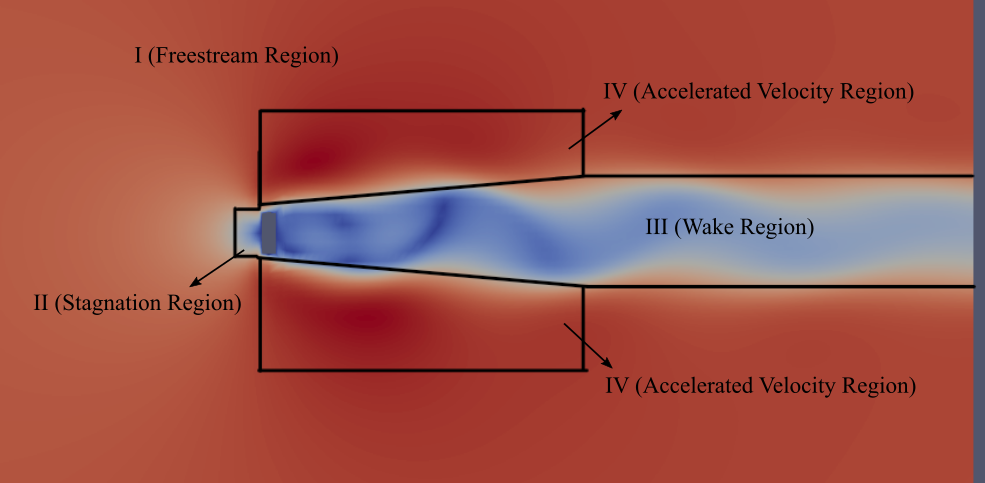
| + | As seen on the zoomed velocity simulation figure above, the result of the simulation is relatively similar to the previous case. However a clear fluid turbulence is visible on the third (wake) region. | ||
Revision as of 21:49, 14 November 2023
Contents
- 1 Introduction
- 2 Numerical Method
- 3 Energy Conversion System
Introduction
- Full Name : Benarido Amri
- NPM : 2106718230
- Major : Mechanical Engineering
- Email : benarido.amri@ui.ac.id
- Lecturer : Dr. Ahmad Indra Siswantara
Assalamualaikum Wr. Wb.
My name is Benarido Amri currently studying Mechanical Engineering at Universitas Indonesia. this page would be a way for me to update the progress of learning Numerical Method and Energy Conversion System.
Numerical Method
Design Project
Pressurized Hydrogen Storage
Hydrogen can be a great alternative for conventional electric vehicle energy source, since it can provide many benefits such as less charge time and cleaner environmental waste. However, the problem we face with hydrogen is the safety concerns regarding its storage method, even though hydrogen is generally safe under normal pressure, it can be a major safety issue when stored at such a high pressure -which is how the hydrogen will be stored in a EVs-, upon accident many worried that the hydrogen could explode, or catch fire.
In this Numerical Method class, our ultimate goal would be to find a way to safely contain pressurized hydrogen. Although we are going to focus on a much smaller case and less pressure. With the specifications being 1 liter of hydrogen pressurized to 8 bar.
Hydrogen Application
Hydrogen is the lightest element in the universe and it can be used for many applications. There are many forms of hydrogen such as liquid form, gaseous form, and even solid form. These form have different uses of their own. Here are some applications for hydrogen according to their various forms:
- Liquid form hydrogen = Liquid form hydrogens are commonly used as a fuel for rocket, where it is used alongside an oxidizer. Apart from rocket fuel, liquid hydrogen can also be used as a fuel for internal combustion engine (ICE) and fuel cell.
- Gaseous form hydrogen = This form of hydrogen can potentially be a great alternative fuel source for vehicles such as cars or trucks.
- Solid for Hydrogen = There is currently a research on the possibility of storing hydrogen as a solid for vehicle fuel.
Optimization Consideration
We were tasked of designing a pressurized hydrogen storage tank which can hold up to 1 liter of 8 bar hydrogen which costs less than Rp. 500 000. For the optimization, we wanted to optimize the cost without sacrificing the performance such as safety, and reliability.
Material Selection
The current material selection for the storage is generally made of metal such as austenitic stainless steel (AISI 316 and AISI 304). This is because hydrogen storage must have very high tensile strength, low density, and doesn't react with hydrogen.
Optimization Objective
- Design Variables = Thickness, weight, and deflection.
- Objective Function = To find the most suitable wall thickness when considering the trade off between weight and strength (deflection) of the storage tank.
- Constraints = The storage tank must be able to fit within a space of 5.8325 cm x 5.8325 cm x 11.0234 cm rectangular box shape or around 1.5 L of volume. And must be able to hold a minimum of 1 L of hydrogen.
For the storage tank project, I will attempt to optimize the wall thickness of the tank by considering the weight and deflection. Weight can be a crucial factor especially when the storage tank is for applications that needs to be mobile and light. However if we were to use the same material, reducing weight can have an effect on its strength, one aspect of strength compromised is its ability to resist deflection when given a force.
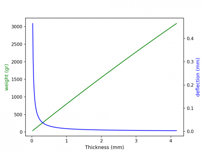
The optimization process is done by using a graph to find the intersection point between deflection and weight. Due to the many formulas and equations involved, we can simplify the calculation by using a code such as python or MATLAB. In my case, I will be using a python programming language.
Design
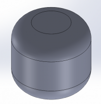
Before we can calculate the weight and deflection, we need to define our material, shape, and also size. The shape of the tank can be divided into 2 basic geometry, the main cylinder and the cap on both sides. The total dimension of the storage tank is 11.0234 cm in length and has a radius of 5.8325 cm. The main cylinder has a height of 5.1909 cm and a radius of 5.8325 cm, while the cap has a radius of 5.8325, a height of 2.91625 cm, and a fillet radius equal to half of the main cylinder radius. These description can be seen on the image below.
The size and shape is taken from Jiddan's work on the ideal radius to height ratio of such storage tank, determining the ideal ratio to be around 1.89.
For the material, from the paper "Materials for hydrogen storage" by Andreas Zuttel, they stated that the common material for hydrogen storage is stainless steel AISI 316 and AISI 304, which is an austenitic type steel. So for the design project I decide to use the stainless steel AISI 304. AISI 304 is quite a common material and it is often used for many applications outside of the storage tank.
Coding
Due to the many variables and formulas involved, coding can be a great tool to help us calculate all the numbers for the graph. The code starts with importing the necessary modules from the library. The next step would be to define the known parameters, in this case the total height, outer radius, cylinder height, total volume, modulus of elasticity, and the simulated force.
We use the the same for loop to calculate all the necessary variables, such as the weight and deflection. Here we have the equations used to calculate the variables shown in figure 2.2.
To calculate the deflection, only the main cylinder is calculated with the assumption of the load situated at the middle of the cylinder. This is to simulate an impact at the center of the tank while the tank is empty and thus there is no pressure acting on the inside of the cylinder. This assumption may not be accurate, however since I couldn't find the appropriate formula for the shape of the whole storage tank, we will need to go by this assumption. The diagram of the calculation can be seen in figure 2.3.
   h_t = 11.0234  # Total height
   r_o = 5.8325  # Outer radius
   h = h_t - r_o  # Cylinder height
   V_t = 1454.8338  # Total volume
   E = 193e9  # Modulus of elasticity for AISI 304
   F = 100000  # Simulated force
   results1 = []
   results2 = []
   results3 = []
   for r_i in np.arange(5, r_o - 0.0025, 0.0025):
       fluid_volume = ((4*(r_i**2)) * h_t) - (pi * (r_i**2) * (4/3 * 1/64 * r_i + 1/16 * h))
       material_volume = V_t - fluid_volume
       weight = material_volume * 8  # Weight is the volume times the density of material (8 gr/cm^3)
       thickness = (r_o - r_i)/2 * 10  # Calculating the thickness in (mm)
       deflection = ((F * (h_t/100)**3)/(48 * E * (pi/64 * (((2 * r_o/100)**4)-((2 * r_i/100)**4))))) * 1000  # Calculation of the deflection converted to (mm)
       results1.append(weight)
       results2.append(deflection)
       results3.append(thickness)
From the code above we can then plot the values into a graph as shown below :
From the graph by finding the intersection between the two lines, we can find the best wall thickness, which is around 0.312 mm. With a weight of 266.7 gram and a deflection value of 0.03775 mm.
Conclusion and Evaluation
Based on the result above, the ideal thickness when considering only the weight and the deflection factor would be 0.312 mm, however we must also consider other factors when designing or manufacturing storage tank. Although the result of the wall thickness seems to be very thin, this is probably due to the assumptions of taking only the wall cylinder.
We can change the wall thickness according to different materials and their properties, a stronger material would reduce the thickness even more whilst weaker material requires thicker wall.
Other interesting note that we can take from this procedure is that it is relatively simple to do, and can be done for many other parameters that we wanted to know, the accuracy however may not be as accurate as some other methods.
For further improvements, I think the best approach is to make the calculations more detail and more realistic, it will also be a great addition if we include simulation such as from ansys, solidworks, or other CAD software. There are some assumptions that might not be ideal for the optimization and also there are some idealization that might not be suitable for this particular case.
As mentioned previously, this approach only accounts for the weight and deflection and not other important factors. Since we are focusing on the optimization aspect of the design process, I only took certain parameters to work on while ignoring other crucial factors. Upon designing and manufacturing a product, we must consider all the factors and must also design according to the code, from its dimensions, safety, reliability, cost, and others.
Conscious Effort
Consciousness is an integral part of our lives, it allows us to have the ability to think, make decisions, and also differentiate between right and wrong. When we are working on this project, there are a lot of decisions and calculations that we have to make, such as at the start where we decide what variable(s) we want to optimize or towards the middle where we think about the code or at the end where we arrive at the conclusion of our project.
All of these different things that we did require a conscious effort, thus it is important for us to recognize and cherish our consciousness. And lastly, we have to be grateful for the opportunity that is given to us to experience our life, and have our own consciousness.
Final Presentation Video
My presentation video about my conscious effort on learning numerical method and its application in hydrogen storage design optimization can be found on the link below:
https://www.youtube.com/watch?v=EdskKzZS2bE
In this class, I have learned a lot about the importance of recognizing my own consciousness "I am my own consciousness" and how significant of a role it plays in our every day lives, from the second we woke up from sleep in the morning to the second we sleep again at night. Consciousness grants us the ability to do things that are integral to our lives, such as deciding between right and wrong, or having the ability to solve complex problems, or the ability to decide between several choices, or the ability learn new things and have many different perspective, and many others.
However, even though consciousness is important in our lives, we sometimes forget how essential it is for our lives, therefore it is important for us to recognize and appreciate our own consciousness and also be grateful of it.
Energy Conversion System
Class Summary (Monday, 30 October 2023)
“Education is what remains after one has forgotten what one has learned in school.”
- Albert Einstein
There are 3 levels of understanding in general, the first level is to first understand the “what”, the second level is about the “how” and lastly is to understand the “why”.
If we apply the 3 levels above to energy, we can answer the “what” question in terms of equation shown below:
dE/dt=W+Q
One of the fundamentals of energy is that it can neither be destroyed nor created, instead, it can only be converted. In practical fluid system application, energy conversion is present in pumps or turbines. To maximize the conversion, we need to understand the importance of efficiency. Efficiency in pumps are the measure of the ratio between the energy at output and at input.
Vertical Axis Wind Turbine (VAWT) CFD Simulation Using CFDSOF
Set Parameter Values
- Start time = 0
- End time = 2
- Inlet velocity = (12 5 0), 12 at the x-axis and 5 at the y-axis
Results
Pressure results
- Pressure Magnitude
The result of the pressure magnitude is presented in figure 3.1.
- Pressure at t = 0.045
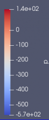
A clear pattern can be seen on figure 3.1 where the difference in pressure is indicated by the colors, where blue indicates lower pressures and the red color indicates higher pressure regions. At the turbine area, a low pressure region can be observed on the near side (relative to the axis of rotation) of the bottom airfoil, and a higher pressure region on the far side (relative to the axis of rotation) of the bottom airfoil.
However, there is a slight abnormality that can be seen at the top middle of the figure 3.2, a lower pressure region which does not seem to be interacting with the simulated object (VAWT).
- Pressure at t = 0.87
At t = 0.87, a similar situation can be observed in the simulation, where there is a clear difference in pressure between the far side and near side of the airfoil.
- Pressure at t = 1.045
A clear difference in pressure is observable, however, in this instance, the higher pressure region is present at the near side of the top right airfoil as opposed to the far side which was the case for the previous 2 timeframe. Furthermore, the most observable pressure difference seems to be when the airfoil is almost at a perpendicular angle to the direction of the wind.
Velocity Results
- Velocity Magnitude
The result of the velocity magnitude is presented in figure 3.1.
- Velocity at t = 0.045
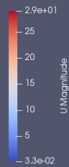
The pattern for velocity changes is much more observable and clearer when compared to the pressure simulation. The color indicators are the same however, where blue indicates lower velocity and red indicates higher velocity. Although the patterns are more observable, it is more difficult to draw a correlation from the result of the simulation.
But there are still some pattern that are observable, such as the velocity profile is relatively turbulent, especially at the longer distances from the airfoils.
Another abnormality is also present in the velocity simulation similar to the previous simulation. It is also at the same exact location as the previous one.
- Velocity at t = 0.87
The turbulent nature of the velocity pattern is much more observable at t = 0.87. Especially at the two bottom airfoils of figure 3.7.
- Velocity at t = 1.045
Similar to the previous timeframe, a turbulent pattern is observable for all airfoils.
Difficulties
Although the intention was to set the end time to 2, due to the high processing power requirement, I was only able to get the time to 1.135.
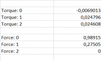
Torque & Force Result
The torque and force results are presented in the figure 3.9.
CFD Simulation Software
In the past, it is often difficult to test a design since we need to have the appropriate testing equipment and then create a prototype from the design. And then, calculations of non-dimensional number such as Reynolds number is required in order to have accurate testing. Furthermore, it is often difficult to decipher all the information based on the testing result.
In the digital age, an alternative method of design testing is available. With the help of simulation software such as CFDSOF, Ansys, SimFlow, Autodesk CFD, and others, testing can be done with relatively minimum effort with much more detailed results. By using simulation software, details such as pressure or velocity at each points on the model can easily be viewed.
Simulation software allows for more efficient and cost effective way to optimize or test a design.
Class Summary (Wednesday, 8 November 2023)
To learn about the simulation, a simplified version of a turbine is used whereby the turbine only has 2 blades. This simplification is in order to learn the basics of the CFDSOF software. It also enables us to understand how the energy is converted following a basic formula of kinetic energy, potential energy, pressure, and velocity.
Static 2-Dimensional Simulation of a Single Blade
Parameters
- Box geometry properties: 1 m X 3 m X 1 m
- Base mesh: 10 m X 10 m X 0.1 m
- Velocity reference value: 0.01 m/s
- Simulation mode: Steady-state, laminar, incompressible
- Initial condition = Fixed value velocity with 0 m/s speed
Result
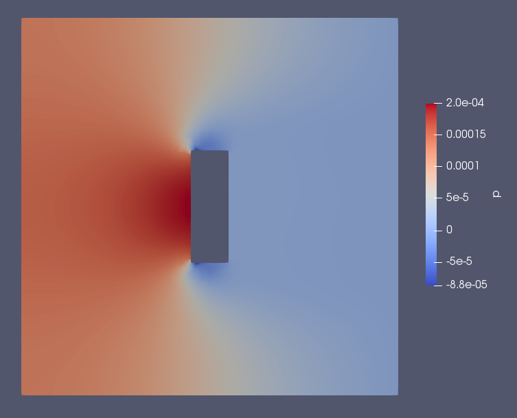
Pressure
From the figure above, a high pressure region is visible at the front side of the blade. These higher pressure region can be one of the causes of the turbine to ultimately rotate on its axis of rotation. Theoretically, the larger the surface area of the blade, the more pressure will develop at the front of the blade. However, larger surface area also means more material is needed thus adding weight as well.
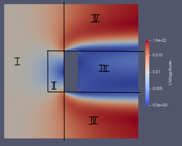
Several interesting points can be drawn from the figure above:
- The left input side is relatively uniform. (Area 1)
- A small area right in front of the blade has 0 velocity. (Area 2)
- The area covered by the blade has relatively low velocity. (Area 3)
- However, the area above and below has a highest velocity amongst the other areas. (Area 4)
The increase in velocity in area 4 can be explained simply as the fluids way of maintaining the same flow rate throughout the control volume. The equation is Q1 = Q2 or V1 * A1 = V2 * A2, because of the obstruction caused by the blade, the area of the control volume decreases, thus to maintain the same output flowrate, the velocity of the air must increase as well. Creating the shape and pattern as seen in the figure above.
Revised Static 2-Dimensional Single Blade Simulation
Parameters
- Box geometry properties: 0.1 m X 0.3 m X 1 m
- Base mesh: 10 m X 10 m X 0.1 m at 200 X 200 X 1 division
- Velocity reference value: 0.01 m/s
- Simulation mode: Steady-state, laminar, incompressible
- Initial condition = Fixed value velocity with 0 m/s speed
Result
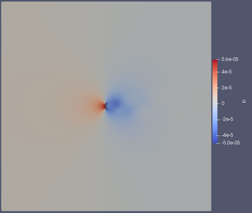
Pressure
Velocity
Due to the much larger ratio between the control volume and blade size, a clear freestream region is visible outside of a certain radius of the blade.
As seen on the zoomed velocity simulation figure above, the result of the simulation is relatively similar to the previous case. However a clear fluid turbulence is visible on the third (wake) region.


