Tanveer khan
Contents
- 1 Predicting Static Stress in One-Dimensional Bar Elements Using Artificial Neural Networks coupled with DAI5 Framework-by-Tanveer Khan
- 2 DAI5 Framework:
- 3 Total deformation analysis of a bar using 1D elements and Ansys 2021R2:
- 4 2D plane stress analysis using Ansys 2021R2:
- 5 Pipe stress analysis using Ansys 2021R2:
- 6 Basic questions:
- 7 2D_beam stress_strain analysis using Ansys 2021R2:
- 8 shell plain stress_strain analysis using Ansys 2021R2:
- 9 Interpretation of Post-Processing Results:
- 10 Finite element equations from a 1D Partial Differential Equation (PDE) using the weighted residual method:
- 11 Algorithm, Flow chart, and python code for a 1D FEM:
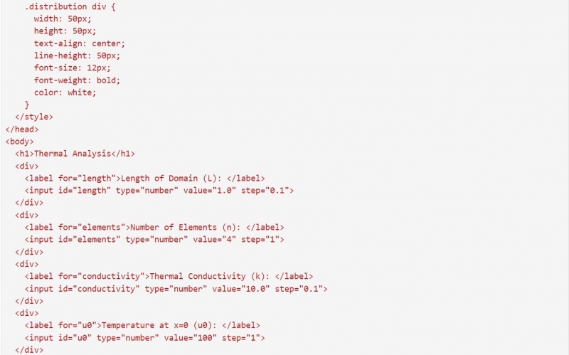
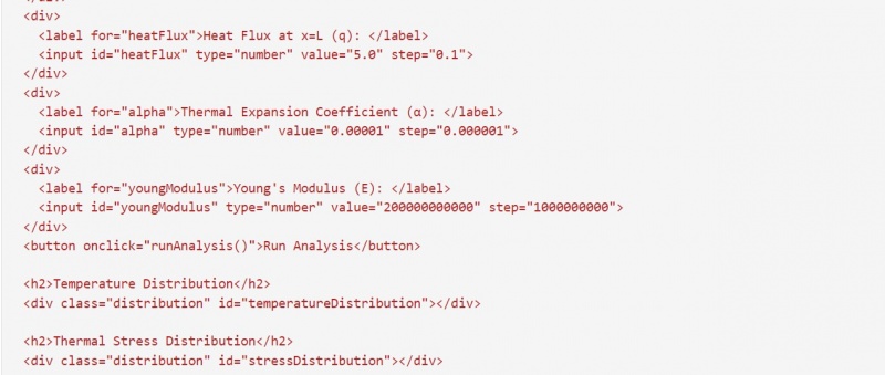
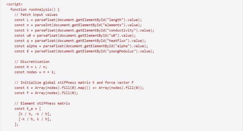
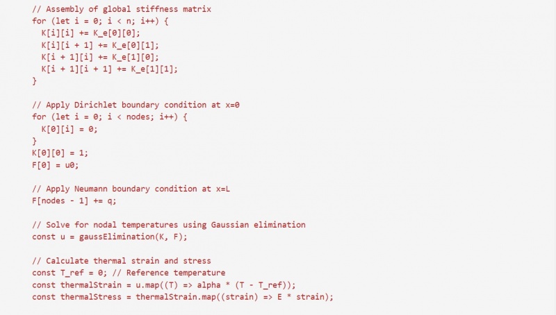
- 12 1D Thermal analysis using web based Java script:
Predicting Static Stress in One-Dimensional Bar Elements Using Artificial Neural Networks coupled with DAI5 Framework-by-Tanveer Khan
Hello! Welcome to my Wiki page.
I am Tanveer khan from Pakistan, studying at the Faculty of Engineering Universitas Indonesia(FTUI). My major is Mechanical engineering and my specialty is manufacturing and automation systems. I've enrolled in a Finite Element and Multiphysics course to gain a deeper understanding of the fundamental principles and applications of FEM, as well as to explore various types of simulations.
DAI5 Framework:
Hello, I am Tanveer Khan presenting the DAI5 Framework, an innovative approach developed by Dr. Ahmed Indra (DAI). This method, DAI5, focuses on intentions, initial thinking, idealizations, and instruction sets for effective problem-solving. I discuss the unique aspects of DAI5 and how it differs from traditional approaches, emphasizing the importance of clarity and specificity in instructions. Viewers are encouraged to understand the significance of setting clear objectives and simplifying complex problems.
Total deformation analysis of a bar using 1D elements and Ansys 2021R2:
2D plane stress analysis using Ansys 2021R2:
Pipe stress analysis using Ansys 2021R2:
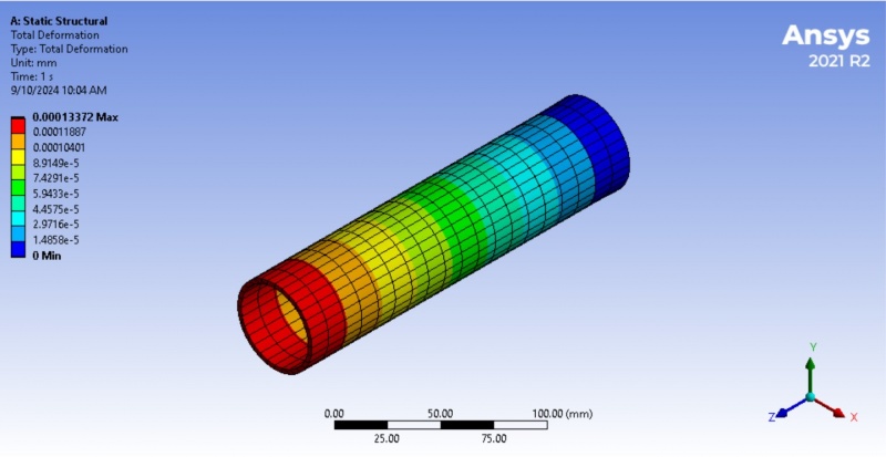
I used the following specifications for the stress analysis of the pipe using the Ansys 2021R2;
Material:
1)Structural steel.
Geometric dimensions:
1) Length: 200mm.
2) Outer Diameter: 50mm.
3) Inner Diameter: 45mm.
4) Thickness: 2.5mm.
Boundary conditions:
1) Fixed right end.
2) Applied load to the left end (Load= 50N).
<<<Total deformation:>>>
The image shows a structural analysis result from ANSYS software. The analysis focused on the total deformation of a pipe under 50 N load. The color gradient ranges from red (maximum deformation) to blue (minimum deformation). Red represents the area with the highest deformation, around 0.00013372 mm. Blue indicates the region with little or no deformation. Based on the image, the highest deformation occurs at the left end of the pipe, which is colored red, while the least deformation occurs at the opposite end, in blue which is 0 mm.
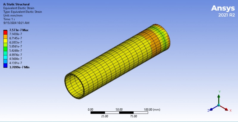
<<<Strain:>>>
The image shows strain analysis results from an Ansys simulation, specifically for a pipe, analyzed using static structural analysis. The result shows the elastic strain distribution in a pipe under 50N load. The maximum strain occurs near the right end of the pipe, possibly due to concentrated stresses, while the rest of the pipe experiences a more uniform, lower strain. The color scale on the left ranges from blue (minimum strain value 3.7099×10^−7) to red (maximum strain value 7.573×10^−7).
Blue/Cyan/Green: These colors represent regions experiencing low to moderate elastic strain.
Yellow/Orange/Red: These regions experience higher elastic strain, with red indicating the maximum strain values.
The highest elastic strain (indicated by red and orange) is located toward the right end of the pipe. This suggests that this portion is undergoing the most deformation under the applied load. On the other hand, the lowest strain (blue) is spread along the middle to the left side of the pipe. This indicates that these areas are relatively less affected by the applied loads, experiencing lower deformation.
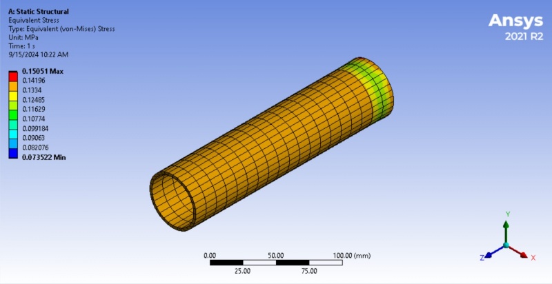
<<<Stress:>>>
The given image shows the result of a finite element analysis (FEA) of a pipe under static structural loading 50N, likely performed in Ansys 2021 R2. The analysis focuses on the Equivalent Stress, specifically the von Mises stress, which is used to predict the yielding of materials under complex loading conditions. The color bar on the left indicates the magnitude of von Mises stress in MPa (megapascals), ranging from 0.073522 MPa (blue) to 0.15051 MPa (red). The color distribution on the pipe shows the areas experiencing different stress levels. Red and yellow areas near the end of the pipe are experiencing the highest stress, while blue and green areas are under lower stress. The highest stress 0.15051 MPa occurs near the end of the pipe, where the colors transition from green to yellow and red. The rest of the pipe has lower stress values, predominantly in the orange-yellow range, indicating that most of the structure is experiencing moderate stress levels. Blue areas, especially on the opposite end, indicate the regions under minimal stress.
Basic questions:
Question(1): Is the force term internal or external in stress-force relation? >>(Sigma= F/A)?
Question(2): Does stress force direction dependent?
Question(3): How do we form the global stiffness matrix based on element-wise stiffness matrices?
2D_beam stress_strain analysis using Ansys 2021R2:
Specifications in (millimeter):
1) Lenght = 4000mm.
2) Wall thickness= 3.4036mm
3) Width= 152.4mm.
Material:
Stainless steel.
Boundary conditions:
1) Simple supported on two ends.
2) Second-end applied Load= 4000N (UDL on 10mm patch in -y direction).
----2D-Stress:----
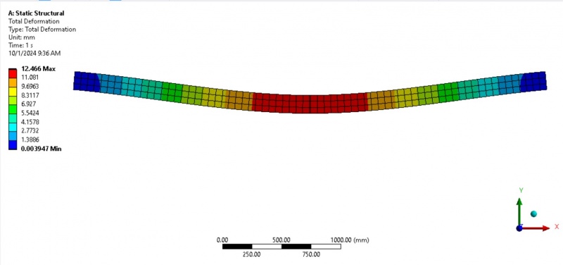
<<<Total deformation:>>>
The given image static structural analysis shows the total deformation of the structure, with a maximum displacement of 12.466 mm in the center (red) and a minimum of 0.003947 mm near the edges (blue). The color gradient from blue to red indicates how the deformation varies, with the highest strain occurring in the middle of the structure, suggesting significant bending or displacement under the applied load. The analysis highlights that the central section is most affected, while the edges experience minimal deformation, reflecting the load distribution across the structure.
<<<Equivalent Stress:>>>
The image shows the results of an equivalent (von Mises) stress analysis for the structure, with the stresses measured in megapascals (MPa). The maximum stress occurs at 300.52 MPa (red), and the minimum stress is 1.0292 MPa (blue). The stress distribution across the structure is represented by a color scale from blue (low stress) to red (high stress), indicating that the areas near the middle of the structure experience the highest stress, particularly in the region with yellow, orange, and red colors. The outer edges, shown in blue, experience the least stress. This type of analysis helps in identifying the most critical areas in the structure that are likely to fail under load. High-stress areas, such as the center, may require design or material changes to avoid failure.
<<<Nomral Stress:>>>
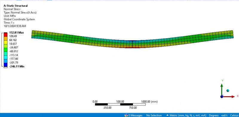
The image presents the results of a normal stress analysis along the X-axis, with stress measured in megapascals (MPa). The maximum normal stress is 152.81 MPa (red), and the minimum is -246.11 MPa (blue). The color gradient, ranging from blue to red, indicates regions of compressive (negative) and tensile (positive) stress, with compressive stress shown in shades of blue and tensile stress in shades of yellow to red. The central area of the structure experiences the most compressive stress (deep blue), while the outer edges near the middle are under the highest tensile stress (red). This distribution suggests that the structure is bending, with tensile stress on the convex side and compressive stress on the concave side, typical for a beam under bending loads.
----2D_Strain:----
<<<Equivalent Elastic Strain:>>>
The image shows the results of an equivalent elastic strain analysis, measured in units of strain (mm/mm). The maximum strain occurs at 0.0067731 (red), while the minimum strain is 3.1269e-5 (blue). The strain distribution follows a similar pattern to the previous analyses, with the highest strain concentrated in the middle portion of the structure (indicated by red and yellow), suggesting this area experiences the most deformation under load. The edges show significantly lower strain (blue areas), indicating less elastic deformation. The color gradient from blue to red shows how strain is distributed across the structure, with the highest strain concentrated in regions of maximum bending. This analysis helps to assess how much the material stretches or compresses elastically, ensuring that the structure remains within its elastic limit to avoid permanent deformation.
<<<Normal Elastic Strain:>>>
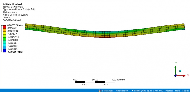
This image displays the results of a normal elastic strain analysis along the X-axis, measured in mm/mm. The maximum normal strain is 0.0025374 (red), and the minimum is -0.0053577 (blue). The distribution of strain is indicated by a color scale, where red to yellow represents tensile strain, and blue to green represents compressive strain. The central region of the structure, particularly in the lower section, shows the highest tensile strain (red and yellow), while the top of the structure exhibits significant compressive strain (blue). This distribution is consistent with the bending behavior of the structure, where tensile strain is concentrated on the convex side and compressive strain on the concave side. The strain values help evaluate the material's elastic behavior and how much deformation the structure undergoes under the applied loads.
shell plain stress_strain analysis using Ansys 2021R2:
<<<Using DAI5 Framework:>>>
<<<Initiator:>>>
The framework is founded and inspired by Prof. Dr. Ahmad Indra.
<<<Intention:>>>
The purpose of this analysis is to study the plain stress and plain strain conditions in a stainless steel cylindrical shell, using a 2D element analysis in ANSYS to examine the stress and strain distribution due to the applied pressure. The objective is to interpret and analyze the following:
1) Normal stress in the x and y directions.
2) Normal elastic strain in the x and y directions.
<<<Initial Thinking about the Problem:>>>
Information Search: I am conducting a 2D element analysis on the shell, which is appropriate for cases involving pressure loading on cylindrical shells.
Nature of the Problem: We are dealing with a static structural problem. The shell is subject to internal pressure, and our interest lies in understanding how this pressure affects the stress and strain fields inside the shell.
Model Specifications:
Length: 2000 mm
Outer radius: 80 mm
Inner radius: 75 mm
Wall thickness: 10 mm
Material Properties: The shell is made of stainless steel, a common choice for high-strength structural applications.
Boundary Conditions:
Pressure: 50 MPa applied on the mid-plane of the shell (acting radially_outward).
Displacement: Free in the x and y directions, fixed in the z-direction.
Support: Cylindrical support allowing radial displacement to be free, but axial and tangential directions are fixed.
<<<Idealization:>>>
Assumptions:
1) The analysis assumes the linear elastic behavior of the material.
2) 2D plain strain conditions are assumed, as the thickness of the shell is relatively small compared to its length.
3) The temperature is the ambient.
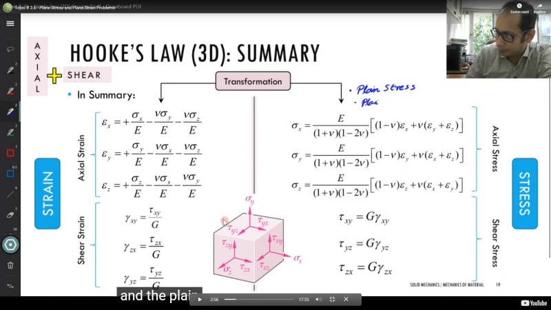
4) Underlying Laws and formulas excluding the z-axis terms from all to get the plain strain-stress as shown in the given picture.
5) Stress-Strain Relationships: Governed by Hooke's law for elastic materials excluding the z_axis terms.
6) Equilibrium Equations: Static equilibrium condition which ensures the structure remains stable under loading.
<<<Instruction Set:>>>
The analysis was conducted in ANSYS 2021R2 using the following procedure:
Model Setup: The geometry of the shell was created using a DesignModeler.
Material Properties: Stainless steel was assigned with appropriate elastic properties.
Meshing: A mesh was generated for the shell to accurately capture the stress and strain distribution by using an element size of 20mm and the Multizone Quad/Tri method.
Boundary Conditions: Radial displacement was allowed, and axial/tangential displacements were fixed as specified. A pressure of 50 MPa was applied.
Solver: Static analysis was performed to compute the stress and strain fields.
Interpretation of Post-Processing Results:
<<<Normal Stress in the x-direction (Sigma_x):>>>
Observation: The normal stress in the x-direction shows a consistent distribution across the shell, with regions of high stress in the center and gradually reducing toward the ends.
Interpretation: The stress in the x-direction is uniform due to the applied boundary conditions and pressure. This stress represents the axial load distributed across the length of the cylindrical shell, peaking at the center where the pressure is concentrated.
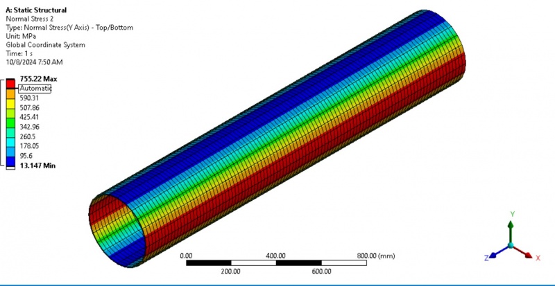
Max Stress: The maximum axial stress is 755.22 MPa.
Min Stress: The minimum axial stress is 13.147 MPa at the ends, which is typical near the constrained boundaries.
<<<Normal Stress in the y-direction (Sigma_y):>>>
Observation: The normal stress in the y-direction also shows a high concentration in the middle, with a gradient decreasing toward the shell's edges.
Interpretation: The circumferential stress arises from the internal pressure applied to the cylindrical shell. The distribution indicates the stress is concentrated in the central region where the load is applied, which is consistent with the pressure application and boundary constraints.
Max Stress: 755.22 MPa, occurring at the mid-plane.
Min Stress: 13.147 MPa, similar to the axial stress behavior near the boundaries.
<<<Normal Elastic Strain in the x-direction (E_x):>>>
Observation: The strain in the x-direction is proportional to the stress distribution, with the highest values appearing near the center and gradually reducing toward the ends.
Interpretation: The axial strain corresponds to the applied stress in the x-direction. The results show higher strain in the middle region of the shell, where the pressure-induced stress is highest. The strain decreases as we move toward the ends of the shell.
Max Strain: 0.0035093 mm/mm showing that the shell experiences significant elastic deformation in response to the applied pressure.
Min Strain: -0.0015275 mm/mm indicating slight compressive strain at the extremities.
<<<Normal Elastic Strain in the y-direction (E_y):>>>
Observation: The strain in the y-direction shows a similar distribution to the x-direction strain, with higher values in the center and lower values toward the boundaries.
Interpretation: This strain corresponds to the circumferential strain due to the applied pressure. The elastic deformation follows the stress distribution closely, indicating the shell's expansion under load.
Max Strain: 0.0035093 mm/mm indicating the shell experiences elastic deformation in the circumferential direction.
Min Strain: -0.0015275 mm/mm representing slight compressive behavior at the shell's ends.
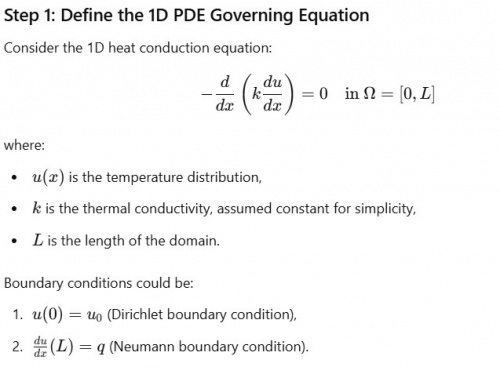
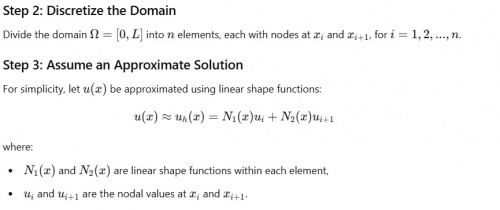
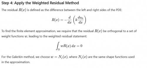
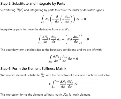
Finite element equations from a 1D Partial Differential Equation (PDE) using the weighted residual method:
I will take the example of a simple 1D PDE for steady-state heat conduction without internal sources.
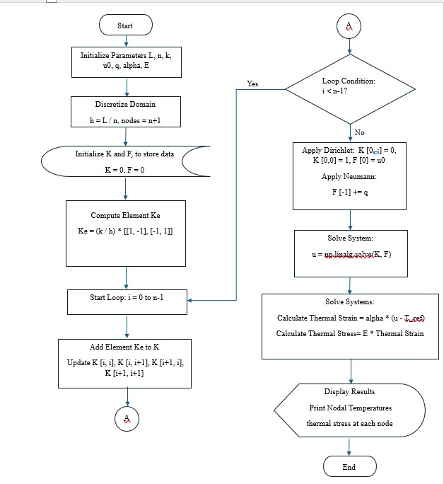
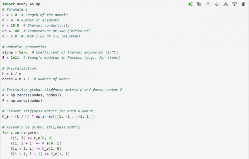
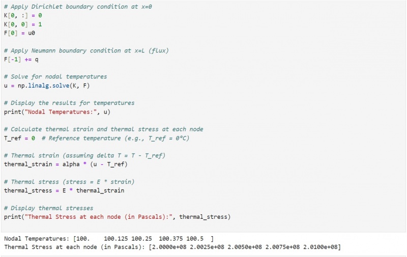
Algorithm, Flow chart, and python code for a 1D FEM:
1) Algorithm:
1) Input the parameters:
>Domain length (L)
>Number of elements (n)
>Thermal conductivity (k)
>(alpha) Coefficient of thermal expansion (1/°C)
>(E) Young's modulus in Pascals
>Boundary conditions at x=0 (Dirichlet) and x=L (Neumann)
2) Discretize the domain:
>Divide L into n elements, each of length h= L/n.
>Define nodes at points x(i)=i.h, for i=0,1,...,n.
3) Construct the element stiffness matrix:
>For each element, calculate the local stiffness matrix K(e)= k/h[[1 -1],[-1 1]]
4) Assemble the global stiffness matrix K:
>Initialize an (n+1)X(n+1) matrix K.
>Add each K(e) to the global matrix K at the appropriate node positions.
5) Apply boundary conditions:
>For Dirichlet (fixed value), set the first row/column in K and F to apply the temperature value.
>For Neumann (flux), modify the last row of F to include the flux value q at x=L.
6) Solve for nodal temperatures u:
>Solve the linear system K⋅u=F to get u (nodal temperatures).
7) Solve for Thermal strain:
>Solve the linear system Thermal strain = alpha * (u - T_ref) to get Thermal Strain (nodal)
8) Solve for Thermal stress:
>Solve the linear system Thermal stress = E * (Thermal Strain) to get Thermal stress (nodal)
9) display the results:
>Nodal Temperatures
>Thermal Stress at each node (in Pascals)
2) Flow Chart:
3) Python code:
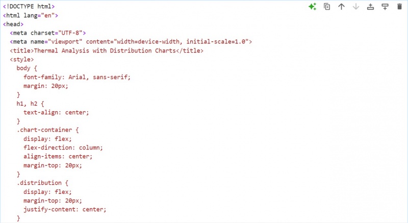
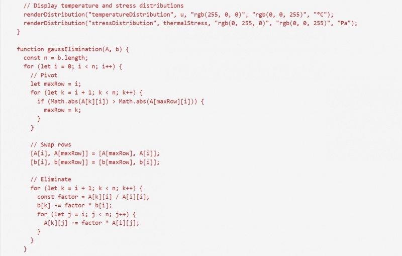
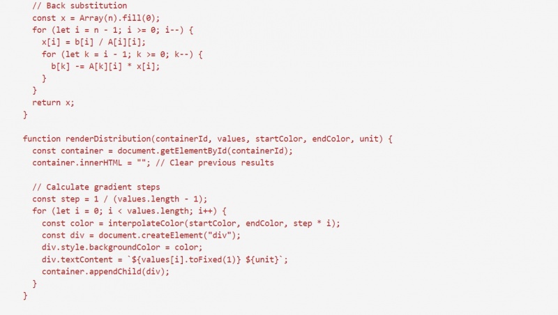
1D Thermal analysis using web based Java script:
1) Javascript:
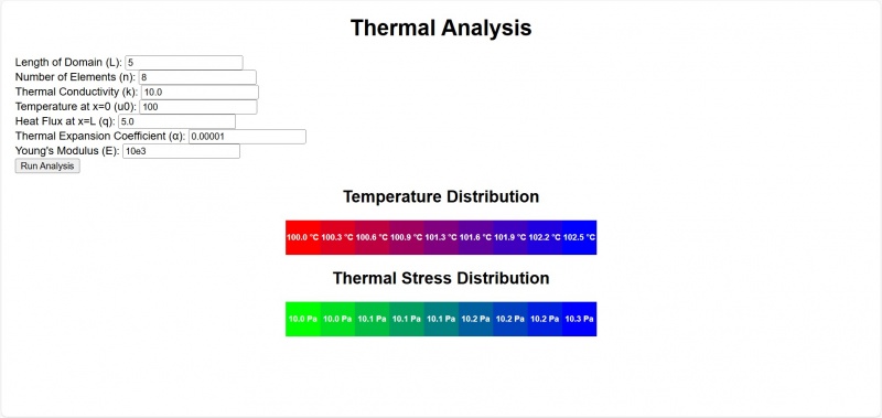
2) Gradient-style bar chart:
