Ardy.lefran
Contents
- 1 Profile
- 2 Engineering Computation
- 2.1 First Class (Feb 3rd 2020)
- 2.2 Second Class (Feb 10th 2020)
- 2.3 Third Class (Feb 17th 2020)
- 2.4 Fourth Class (Feb 24th 2020)
- 2.5 Fifth Class (Mar 2nd 2020)
- 2.6 Sixth Class (March 9th 2020)
- 2.7 Seventh Class (March 16th 2020)
- 2.8 UTS (March 23rd 2020)
- 2.9 Ninth Class (April 6th 2020)
- 2.10 Tenth Class (April 13th 2020)
- 2.11 Eleventh Class (April 20th 2020)
- 2.12 Twelfth Class (April 27th 2020)
- 2.13 Thirteenth Class (May 4th 2020)
- 2.14 Fourteenth Class (May 11th 2020)
- 2.15 UAS (June 8th 2020)
- 3 References
Profile
Fullname: Ardy Lefran Lololau
Nickname: Ardy
Place, Date of Birth: Kupang, August 20th 1997
NPM: 1906433556
Department/Specialization: Mechanical Engineering / Design and Product Manufacturing
Promotor: Prof. Dr. Ir. Tresna Priyana Soemardi, M.Si., S.E. (TPS)
Research interest: Composite materials
Phone: +62 822 47033 572
E-mail: ardy.lefran@ui.ac.id ; ardylefranlololau@gmail.com
Engineering Computation
Courses name: Engineering Computation
Courses code: ENME802004
Lecturer: Dr. Ir. Ahmad Indra Siswantara (Mr. DAI)
Weighting: 2 SKS
Term: 2
First Class (Feb 3rd 2020)
A. What is engineering computation?
In my opinion, engineering computation is an engineering science that uses computer assistance to help an engineer to process a data which complex, repeated, and consists in large numbers, to reduce human error and make time and cost more efficient in solving an engineering matter.
B. What is the objective of this course?
1. To understand the concepts and principals in engineering computation. The terms (iteration, validation, verification, regression, error, convergent, etc.), function, used numerical method, etc.
2. To be able to apply the understanding of engineering computation in a real engineering matter, mainly mechanical. Able to identify a problem, translate it into a programming language (INPUT), use a software on a computer to cultivate it (PROCESS), get a result (OUTPUT) and match it with existing theory.
3. To be a media to know ourselves. Able to identify ourselves (am I confirm with the standard?) in a certain way to get a better understanding in capability of skills, value, and knowledge, especially at engineering computation.
C. Engineering computation capabilities (Muhasabah)
My capability at engineering computation is superficial. I am not really used to engineering computation. My only decent work with engineering computation was the work on my final project at the Bachelor degree, which is using only Ms. Excel to calculate and analyze the amount of dissipation energy that occurs in a composite specimen during a dynamic-tensile test. I am looking forward to learning a lot in this course to improve my skills, value, and knowledge. Credits to Mr. DAI for letting me and my fellow student-friends to have an opportunity to join in this course, and for the insight given to us, hopefully, it will be useful.
Second Class (Feb 10th 2020)
A. Class Resume
In this class, we have been taught again about fundamental things in life. Mr. DAI said that we, as a millennial generation, should not forget nature. We have to study independently like Khairul, a person who has no formal education background but can make and fly his plane. We have to learn from experience because, as the proverb said, the experience is an excellent teacher.
We also have been taught what analysis is. According to the class’s consensus, analysis is an investigation process that includes some activities to solve problems by being reviewed as well as possible using structured thinking. Meanwhile, according to Mr. DAI, analysis is a rational way of the thinking process to gain a matter-solving procedure.
B. Bachelor thesis project with engineering computation
My intention is to implement engineering computation to make a failure model based on the stress distribution of a random-oriented fiber composite, which is i found very hard since the data will spread stochastically. The presence of an open-hole in the middle of the specimen was made the stress concentration localize at it. So I want to make a model of stress concentration factor at the open-hole area. My alternative eagerness is to create a deterministic failure model based on the temperature evolution behavior near the open-hole so that we can predict when the failure is about to occur based on the experimental data. I still have not determined yet which numerical analysis I will use since I am not really used to engineering computation. I will discuss any further with Mr. DAI to guide me for this project.
Third Class (Feb 17th 2020)
A. PPT of Project Synopsis
B. Class Resume
In this class, Mr. DAI tells us to against the nescience, selfishness, laziness. Just like the Police of RI with their slogan "Turn back Crime". In my opinion, one of the ways to against the previous matter is to think critically.
We found a y as x function, as follow: y = (x^2-1)/(x-1). With x = 1, how was the y? If we put the direct substitution into the function, it will conclude y = undefined (0/0). If we change x to 2, 3, 4, and so on, it will culminate y as a real number. So what is the problem?
As human beings, we have to think critically to solve the problem. Back in the math lecture, we have been taught about the limit. In mathematics, a limit is a value that a function (or sequence) "approaches" as the input (or index) "approaches" some value. Thus, if we use limit into the function before, we can see that:
lim┬(x-1)〖(x^2-1)/(x-1)= ((x+1)(x-1))/((x-1))=x+1=1+1 ≈2〗
Fourth Class (Feb 24th 2020)
A. PPT of Project Modelling
B. Quiz
C. Class Resume
FINITE ELEMENT, FINITE DIFFERENCE, AND FINITE VOLUME [1]
The finite-element method is a computational method that subdivides a CAD model into tiny but finite-sized elements of geometrically simple shapes. The next step is to take a system of field equations, mathematically represented by partial differential equations (PDEs) that describe the physics you are interested in, and formulate these equations for each element. This is handled by approximating the fields within each element as a simple function, such as a linear or quadratic polynomial, with a finite number of degrees of freedom (DOFs). When the contributions from all elements are assembled, you end up with an extensive sparse matrix equation system that can be solved by any of several well-known sparse matrix solvers. The type of solver used depends on the original physics since each sort of physics gives its unique imprint on the structure of the matrix. To speed things up, this structure is exploited by using a tailored numerical method.
The finite-difference method is the most direct approach to discretizing partial differential equations. You consider a point in space where you take the continuum representation of the equations and replace it with a set of discrete equations, called finite-difference equations. The finite-difference method is typically defined on a regular grid, and this fact can be used for very efficient solution methods. The method is therefore not usually used for irregular CAD geometries, but more often for rectangular or block-shaped models.
The finite-volume method is similar to the finite-element method in that the CAD model is first divided into tiny but finite-sized elements of geometrically simple shapes. The finite-volume method is based on the fact that many physical laws are conservation laws—what goes into one cell on one side needs to leave the same cell on another side. Following this idea, you end up with a formulation that consists of flux conservation equations defined in an averaged sense over the cells.
Fifth Class (Mar 2nd 2020)
Optimization of Human Energy Needs
People do need energies to have their daily activities, which is commonly called by calories. A calorie is a unit of energy that widely used in terms of nutrition, while in terms of physics, one calorie is the amount of heat energy needed to raise the temperature by 1 °C in 1 gram of water. The amount of calories needed by a person depends on their age, sex, weight, height, and levels of activities.
I am 22 years old men, have 80kg weight, and 175cm height, with a medium level of activities, so according to Harris-Benedict formula, my total calorie needs per day is: (66.5 + (13.75×80) + (5.003×175) - (6.755×22)) × 1.3 = 2461.44 cal ≈ 10.3 kJ
My energies audit for last 1 week can be seen at UTS section. Our class also has been conducted a joint assignment on Optimization of Human Energy Needs.
Sixth Class (March 9th 2020)
A. Class Resume
In this class, Mr. DAI asked us to do the second muhasabah to introspect what we have learned through out the 5 previous class. Mr. DAI also asked us to give ourselves a score to describe the progress. Then we have write it out in paper and to be collected later.
Mr. DAI then told us that now engineering computation has became more relevant, since it has a lot driving force to an engineer to get a wider field to dig in. He also taught us to do what if analysis to get a comprehensive solution for an engineering matter.
At the end of the class, Mr. DAI explained the Rule of Thumb to solve an engineering matter in terms of our engineering computation project. He intended us to make a paper of our case study. The explanation as follows:
1. Initial thinking (Introduction). Knowing the unknown and set the objective.
2. Modelling. Develop the model based on assumption and relevant theory.
3. Analytical work. Do simulation (run the developed model). In this stage, make sure that we do verification and validation. Verification is numerical error checking to resolve the equation (model) right. While validation was done to get the actuality of the model in terms resolving the right equation (model).
4. Result & Discussion. Result got from the analytical work is being discussed to gain a better understanding in resolving an engineering problem.
5. Recommendation. Finally get the solution done and recommend it for the future works.
6. References. Do not forget to show the cited references.
Seventh Class (March 16th 2020)
There is no actual class in this week, due to the UI Rector's circular letter regarding remote learning related to efforts to prevent international pandemics COVID-19 outbreaks. Students are given the task to continue main tasks regarding the bachelor thesis project using engineering computation.
As progress, I am still working on the model of stress concentration factors in the hole area of Lontar fiber composite which about to be posted later next weeks.
UTS (March 23rd 2020)
Learning outcomes video
Energy audit report
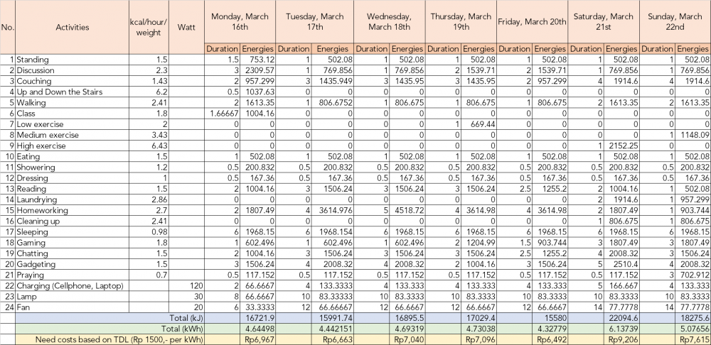
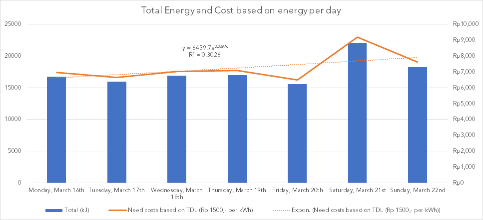
Based on the class joint assignment on Optimization of Human Energy Needs, there is my energies audit for last 1 week (March 16th - March 22nd):
Engineering computation project paper draft
Discussion page [Paper draft]
Ninth Class (April 6th 2020)
Today class is a [Paper draft] presentation.
Tenth Class (April 13th 2020)
Quiz
Eleventh Class (April 20th 2020)
Today's class was an article collaboration group discussion regarding Oscillating one-dimensional system. My group got a ration discuss about Using Python Software to Resolve ODEs on Oscillating Mechanical Systems. Then we were told to choose one other method to solve the Oscillating Mechanical System ODEs. After a comprehensive discussion, my group decided to use the ANN (artificial neural network) method.
Artificial Neural Networks (ANN) are the pieces of a computing system designed to simulate the way the human brain analyzes and processes information. They are the foundations of Artificial Intelligence (AI) and solve problems that would prove impossible or difficult by human or statistical standards. In this section we will show the steps of solving the one-dimensional oscillating body case mentioned above using Neural Network/Data manager (nntool) on MATLAB. Firstly, we set the time variable as the input and the displacement and velocity variable as the targets on the MATLAB Editor task, imported from the discrete data by the Analytical Method. After running the complete syntax on the Editor task, the input and target variables can be set, then we make a new network in Neural Network/Data manager (nntool) menu. Then we start training the network, so that the result of output and error data can be seen.
Twelfth Class (April 27th 2020)
In this class, we have an assignment to get to know ourselves better in explaining an understanding of the principles and concepts in engineering computation. What I understand the most during the course of engineering computation was that we as engineers must be able to find a problem and translate it into a mathematical model to be solved in an initial thinking phase.
The problem that I found is that a representation of an analytic curve in a CAD system.
We found that an analytic non-parametric curve has an equation by: y - y1 = ((y2 - y1)/(x2 - x1))(x - x1). This equation will not satisfy all curve condition, as a vertical curve (parallel to y axis) will have an infinity gradient.
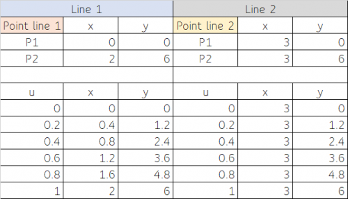
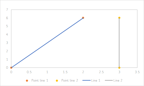
For example we got line 1 connected by 2 coordinate points p1(0, 0) and p2(2, 6). According to analytic non-parametric curve equation, this line do have a define gradient by solving the equation, resulted in y = 3x.
But for line 2 connected by p1(2, 0) and p2(2, 6), will resulted in y equal infinity of x, which can not be processed by computers.
To solve this problem, we have to add a parameter u, as a variable to x and y. Hence the equation becomes: x(u) = x1 + (x2 - x1)u and y(u) = y1 + (y2 - y1)u, where 0≤u≤1, we called this as an analytic parametric equation, and will satisfy all curve condition, also can be read easily by computers.
To provide a clearer picture, I have made a simple simulation of this parametric analytic curve using Ms Excel.
With this equation, we are able to find the mid point of the curve by simply put u equal 0.5, as the computers usually provides. We also able to multiple the length of the line by multiplying u as we desired.
Thirteenth Class (May 4th 2020)
In today class we got an assignment to translate a paper entitled "Simplified Finite Elements model to represent Mass-Spring structures in dynamic simulation" by Rúbia M. Bosse and André Teófilo Beck. Our group has been assigned to translate the 4.1 section regarding 1-storey frame under an impulse force. This paper presents the stages of the deduction approach to making a simple finite element model, to get the results obtained with the mass-spring (MS) model. The main objective is to show the limitations of each model used and to facilitate comparisons between numerical results obtained with different models. Examples of applications are vibration control systems, theoretical model analysis, component modeling mechanisms. This paper presents the hypotheses needed to construct a hierarchical model, discussing the effect of each assumption or simplification in structural responses. With this goal in mind, computer coding is implemented to complete the 2D framework structure under dynamic load with a bulk spring model and finite element model positions considering nonlinear geometric analysis. The results showed that the hypothesis proposed was sufficient to reproduce in the FE the same response method from the MS model experiencing earthquake impulses and loads.
Fourteenth Class (May 11th 2020)
Today's class we discuss a case of basic mechanics where when the area 𝐴 (mm2) is enlarged, the amount of the force 𝐹 (N) increases too, whereas why does the pressure drop ∆𝑝 (MPa) decrease when the area 𝐴 is enlarged?
To answer this, I begin by assuming a work object is experiencing friction, then the applicable mechanical equation is:
𝜏 = 𝐹/𝐴 (1)
Where 𝜏 is the shear stress (MPa).
If the work object that is experiencing friction is a fluid that works in a pipe, then the equation becomes:
∆𝑝 = (𝑓 𝐿 𝜌 𝑉^2)/(2 𝐷) (2)
Where 𝑓 is the friction factor, 𝐿 is the length of the pipe (m), 𝜌 is the fluid density (g / cc), 𝑉 is the flow velocity (m / s), and 𝐷 is the pipe diameter (mm).
If Equation 1 is transformed into force basis, then the equation becomes:
𝐹 = 𝜏 𝐴
Thus it can be seen that by increasing the area of 𝐴, the amount of the force 𝐹 will also increase, with a note that the shear stress 𝜏 remains or does not decrease. Because it has the same dimensions MPa (pressure), for this case, I tried to replace the shear stress with the pressure drop in Equation 1. Then it can be clearly seen that the value of the pressure drop will decrease along with the increase in the area of 𝐴, if the amount of the force 𝐹 remains.
If we combine these two equations,
(𝑓 𝐿 𝜌 𝑉^2)/(2 𝐷) = 𝐹/𝐴
It can be seen that by increasing the area of 𝐴, the diameter of the pipe 𝐷 will automatically increase, because the area of 𝐴 is a quadratic function of the diameter of the pipe 𝐷. As the diameter of the pipe increases, while the friction factor, the density of the fluid, the length of the pipe does not change, the pressure drop ∆𝑝 will decrease.
A little extra, as the value of the pipe diameter and area increases, the flow velocity will decrease, based on the fluid continuity equation,
𝐴_1 𝑉_1 = 𝐴_2 𝑉_2
(as explained by Dieter earlier) which causes the value of the pressure drop to decrease further.
UAS (June 8th 2020)
Excel file: https://drive.google.com/file/d/1UC3qlCgjYTeE6ilEDgopdWSXB4Uz2o58/view?usp=sharing


