Mekanika Fluida - Josiah Enrico S (1906356286)

Title: Modelica-based Simulation of Viscous Flow Through Pipes Using Finite Element Formulation

Multiple Pipe System Example

Abstract

As the piping system has always become an integral part of any fluid-related mechanical system, controlling and measuring the flow properties, such as pressure, flow rate and Reynolds number inside the pipe is a necessary field to master in order to engineer the efficient arrangement. These properties are critical and can be analytically computed by considering fluid factors like density or viscosity and the pipe dimension. Unfortunately, this current method is not scalable since it is examined too onerous and time-consuming to address complex systems. On the other hand, many numerical method programming has been developed to help engineers overcome those problems. This white paper will recreate one simple problem of a multiple pipes system utilizing Modelica programming language and compare it with the current analytical technique to verify the results. This simulation is expected to be a base in developing a scalable program for multiple pipe systems in further work.

Background and Problem Introduction

• Background Theory (Saeed Moavani)

Direct Formulation of Flow Through Pipes

The internal flow through a conduit may be classified as laminar or turbulent flow. In laminar flow situations, a thin layer of dye injected into a pipe will show as a straight line. No mixing of fluid layers will be visible. This situation does not hold for turbulent flow, in which the bulk mixing of adjacent fluid layers will occur. Laminar flow typically occurs when the Reynolds number of the flowing fluid is less than 2100. The Reynolds number is defined as

where r and m are the density and the dynamic viscosity of the fluid respectively. V represents the average fluid velocity, and D represents the diameter of the pipe. The flow is said to be in a transition region when the Reynolds number is typically between 2100 and 4000. The behavior of the fluid flow is unpredictable in the transition region. The flow is generally considered to be turbulent when the Reynolds number is greater than 4000. The conservation of mass for a steady flow requires that the mass flow rate at any section of the pipe remains constant according to the equation

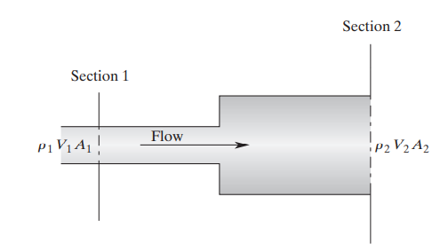
Again, r is the density of the fluid, V is the average fluid velocity at a section, and A represents the cross-sectional area of the flow as shown in the figure below.

For an incompressible flow—a flow situation where the density of the fluid remains constant, the volumetric flow rate Q through a conduit at any section of the conduit is also constant:

For a fully developed laminar flow, there exists a relationship between the volumetric flow rate and the pressure drop P1 - P2 along a pipe of length L. This relationship is given by

---

Finite Element Formulation (Saeed Moavani)

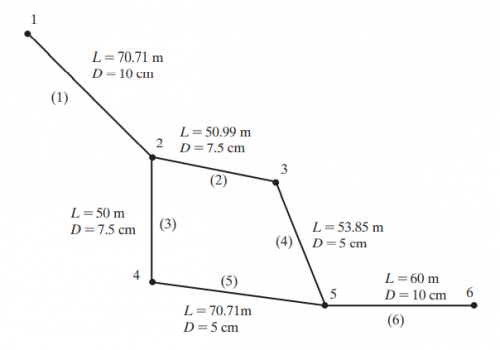
Consider an incompressible laminar flow of a viscous fluid through a network of piping systems, as shown in the figure below. We start by subdividing the problem into nodes and elements. This example may be represented by a model that has four nodes and four elements

The behavior of the fluid flow inside a pipe section is modeled by an element with two nodes. The elemental description is given by the relationship between the flow rate and the pressure drop as given by this equation, such that

where the flow-resistance coefficient C is given by

Because there are two nodes associated with each element, we need to create two equations for each element. These equations must involve nodal pressure and the element’s flow resistance. Consider the flow rates Qi and Qi+1 and the nodal pressures Pi and Pi+1 of an element, which is related according to the equations

The equations given by (12.16) were formulated such that the conservation of mass is satisfied as well. The sum of Q(i) and Q(i+1) is zero, which implies that under steady-state element conditions, what flows into a given element must flow out. Equations can be expressed in matrix form by

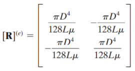
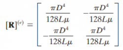
The element’s flow-resistance matrix is then given by

Applying the elemental description given by Eq. (12.17) to all elements and assembling them will lead to the formation of the global flow matrix, the flow-resistance matrix, and the pressure matrix.

---

• Problem Introduction

Example 12.1

Oil with a dynamic viscosity of m = 0.3N∙s/m2 and density of r = 900 kg/m3 flows through the piping network shown in the Figure above. The 2–4–5 branch was added in parallel to the 2–3–5 branch to allow for the flexibility of performing maintenance on one branch while the oil flows through the other branch. The dimensions of the piping system are shown in Figure 12.6. Determine the pressure distribution in the system if both branches are on line. The flow rate at node 1 is 5 * 10-4 m3/s. The pressure at node 1 is 39182 Pa (g) and the pressure at node 6 is -3665 Pa (g). For the given conditions, the flow is laminar throughout the system. How does the flow divide in each branch??

Objectives

The objectives of this study are as follows:

1. Develop a Modelica-based simulation to compute the pressure, flow rate, and Reynolds numbers in the selected points.
2. Validate the results with the corresponding resources.
3. Verify the results with the parameters and boundaries.

Methodology

• The Analytical Calculation

Based on the formula analysis above, we can first determine the local elemental flow resistance in each of 6 points. The matrix can be written as

And the local matrix of the 6 points or nodes are

Then, we can sum up all the local elemental matrices into the global resistance matrix. So, we obtain

Applying the boundary condition and making matrix equation, we have

Solving the simultaneous algebra system using Gauss Jordan, we have the pressure as follows

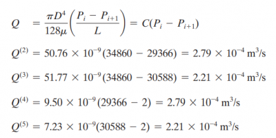
And the flowrate distribution in each pipe are

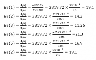
In addition, we could also calculate the Reynolds number as follows

• The Simulation Program

This program is separated into two sections, the first one is the definition phase where the operator needs to input all the properties and the pipe geometry at once. There are 2 fluid properties considered which are dynamic viscosity (N∙s/m2)to calculate the head loss and the density (kg/m3) to calculate the Reynolds number. To set the limit point and boundary condition, the measured pressure (Pa) at the inlet and outlet are also defined at point 1 and 6. Afterward, the parameter of piping like its diameter and installed distance are collected using 2 column matrix. The additional data of Q inlet or point 1 is used to verify the result at the end of the simulation.

The second section is the algorithm section where those data are processed into the requested solution. This step will include the steps mentioned in the analytical calculation above starting from making the local 4x4 matrix of elemental flow resistance, combining them to one global 6x6 matrix, applying boundary conditions, and finally computing the pressure at 6 points also flow rate and Reynolds number at 6 connected pipes.

model Tugas_Besar_Mekflu // ==================================== DEFINITION PHASE ==================================== parameter Real miu = 0.3 "dynamic viscosity"; parameter Real rho = 900 "density"; parameter Real Qinlet = 5e-4 "flow rate inlet"; parameter Real Pinlet = 39182 "pressure inlet"; parameter Real Poutlet = -3665 "pressure inlet"; parameter Integer boundary[:] = {1, 6} "Boundary Point"; parameter Integer nPipe = 6 "number of piping"; parameter Integer nPoint = 6 "number of point connected"; final constant Real pi=2*Modelica.Math.asin(1.0); //Inputing pipe connection, length (L) and diameter (D) parameter Real data[nPipe,2] = [ 70.71, 0.1  ; 50.99, 0.075 ; 50 , 0.075 ; 53.85, 0.05  ; 70.71, 0.05  ; 60 , 0.1 ]; parameter Integer no[nPoint,2] = [ 1, 2; 2, 3; 2, 4; 3, 5; 4, 5; 5, 6]; //Solution Real Pressure[nPoint], Flowrate[nPipe], Reynolds[nPipe]; protected Real g[nPoint,nPoint], G[nPoint,nPoint], id[nPoint,nPoint]=identity(nPoint), P[nPoint], Res; // ==================================== SOLUTION PHASE ==================================== algorithm //Iterating to create global matrice for i in 1:nPipe loop Res:= pi*data[i,2]^4/(128*data[i,1]*miu); g:=zeros(nPoint,nPoint); g[no[i,1],no[i,1]]:= Res; g[no[i,1],no[i,2]]:= -Res; g[no[i,2],no[i,1]]:= -Res; g[no[i,2],no[i,2]]:= Res; G:= G+g; end for; //Implementing boundary for i in boundary loop for j in 1:nPoint loop G[i,j]:= id[i,j]; end for; end for; //Solving pressure in each point connected P[boundary[1]]:= Pinlet; P[boundary[2]]:= Poutlet; Pressure:= Modelica.Math.Matrices.solve(G,P); //Solving flowrate in each pipe for i in 1:nPipe loop Flowrate[i]:= pi*data[i,2]^4/(128*data[i,1]*miu)*(Pressure[no[i,1]]-Pressure[no[i,2]]); end for; //Solving Reynolds Number in each pipe flow for i in 1:nPipe loop Reynolds[i]:= 4*rho*Flowrate[i]/(pi*miu*data[i,2]); end for; end Tugas_Besar_Mekflu;

Result and Analysis

The simulation results are:

• Validation

The validation of the simulation results can be proved when we compare them with the analytical results derived from a matrix formulation. This analytical method was discussed by Moavani (2008) and the comparison between them shows almost one hundred percent of acceptance. The deviation of those numbers is relatively small and only resulted from rounding. Thus, if the analytical results are correct, we could validate the simulation is accurate.

• Verification

The verification of the simulation can be observed between the measured flowrate at the first node or the inlet before the calculation and the flowrate results. At first, the flow rate defined as 5 x 10^-4 m3/s. But at the end of the simulation, we get 0.000500018. These number is quite similar therefore it verify the simulation results.

Conclusions

In conclusion, the Modelica-based simulation of multiple pipe systems using Finite Element Formulation (FEA) is feasible and, since the result is validated by other references and verified by the boundary condition, it gives satisfactory results. This study also shows that using a computer-aided numerical method is more time-efficient and recommended to solve complex engineering challenges. The writer hoped that the methodology used in this study can be adopted for further research in the future.

Acknowledgement

This study is a final assignment in the Fluid Mechanics subject at the Department of Mechanical Engineering, University of Indonesia. The writer would express gratitude for Dr. Ir. Ahmad Indra Siswantara, as this paper's advisor, and all other students for providing valuable discussion during the writing period.

References

• Gerhart, P. M., Gerhart, A. L., & Hochstein, J. I. (2015). Munson, young and okiishi’s fundamentals of fluid mechanics (8th ed.). Nashville, TN: John Wiley & Sons.
• Moaveni, S. (2014). Finite element analysis: Theory and application with ANSYS, global edition (4th ed.). London, England: Pearson Education.