Difference between revisions of "Daniswara Azka Surjaatmadja"
| Line 93: | Line 93: | ||
Pada pertemuan kedua Pak DAI menginstruksikan kepada mahasiswa untuk mencari perbedaan dalam pengetahuan dan pola pikir mahasiswa teknik mesin antara mahasiswa S1, S2, dan S3. Dalam menjawab persoalan tersebut Pak DAI mengarahkan agar pencarian dibantu menggunakan ChatGPT. Adapun hasil dari diskusi dengan ChatGPT sebagai berikut ini. | Pada pertemuan kedua Pak DAI menginstruksikan kepada mahasiswa untuk mencari perbedaan dalam pengetahuan dan pola pikir mahasiswa teknik mesin antara mahasiswa S1, S2, dan S3. Dalam menjawab persoalan tersebut Pak DAI mengarahkan agar pencarian dibantu menggunakan ChatGPT. Adapun hasil dari diskusi dengan ChatGPT sebagai berikut ini. | ||
| − | '''User Question :''' | + | '''User Question :''' Give me a question, the question is in three level of degree. One for an undergraduate student, two for a magister student, and three for doctoral student. The question context must be related to mechanical engineering. |
'''ChatGPT Answer :''' | '''ChatGPT Answer :''' | ||
| Line 116: | Line 116: | ||
'''1. Depth of Understanding:''' | '''1. Depth of Understanding:''' | ||
| + | |||
Undergraduate Level: The question focuses on foundational principles, expecting a basic understanding of concepts like energy conservation within a closed system. It doesn’t require detailed technical calculations or modeling, only a conceptual explanation with an everyday example. | Undergraduate Level: The question focuses on foundational principles, expecting a basic understanding of concepts like energy conservation within a closed system. It doesn’t require detailed technical calculations or modeling, only a conceptual explanation with an everyday example. | ||
Magister Level: The question requires a deeper understanding and practical application of heat transfer modes (conduction, convection, radiation). Here, students need to analyze specific engineering problems, consider optimization, and balance cost with effectiveness, demonstrating a more technical grasp. | Magister Level: The question requires a deeper understanding and practical application of heat transfer modes (conduction, convection, radiation). Here, students need to analyze specific engineering problems, consider optimization, and balance cost with effectiveness, demonstrating a more technical grasp. | ||
| Line 121: | Line 122: | ||
'''2. Complexity of Analysis:''' | '''2. Complexity of Analysis:''' | ||
| + | |||
Undergraduate Level: Analysis is relatively simple, mainly focused on explaining core principles and basic applications. | Undergraduate Level: Analysis is relatively simple, mainly focused on explaining core principles and basic applications. | ||
Magister Level: Analysis becomes more complex, involving multi-mode heat transfer, cost considerations, and practical engineering trade-offs. | Magister Level: Analysis becomes more complex, involving multi-mode heat transfer, cost considerations, and practical engineering trade-offs. | ||
| Line 126: | Line 128: | ||
'''3. Scope of Application:''' | '''3. Scope of Application:''' | ||
| + | |||
Undergraduate Level: The application is broad and general, aimed at helping students recognize thermodynamics concepts in everyday scenarios. | Undergraduate Level: The application is broad and general, aimed at helping students recognize thermodynamics concepts in everyday scenarios. | ||
Magister Level: Application focuses on a specific, practical engineering system (e.g., an insulated pipeline) where students must apply advanced knowledge to optimize real-world solutions. | Magister Level: Application focuses on a specific, practical engineering system (e.g., an insulated pipeline) where students must apply advanced knowledge to optimize real-world solutions. | ||
| Line 137: | Line 140: | ||
1. Apa hukum dasar yang digunakan untuk mendeskripsikan aliran panas dalam konduksi satu dimensi? | 1. Apa hukum dasar yang digunakan untuk mendeskripsikan aliran panas dalam konduksi satu dimensi? | ||
| + | |||
A. Hukum Newton | A. Hukum Newton | ||
B. Hukum Stefan-Boltzmann | B. Hukum Stefan-Boltzmann | ||
| Line 143: | Line 147: | ||
2. Pada konduksi panas satu dimensi dalam kondisi tunak, bagaimana perubahan suhu terhadap waktu? | 2. Pada konduksi panas satu dimensi dalam kondisi tunak, bagaimana perubahan suhu terhadap waktu? | ||
| + | |||
A. Suhu meningkat seiring waktu | A. Suhu meningkat seiring waktu | ||
B. Suhu berkurang seiring waktu | B. Suhu berkurang seiring waktu | ||
| Line 149: | Line 154: | ||
3. Kondisi batas tipe Dirichlet pada masalah konduksi panas satu dimensi menyatakan bahwa: | 3. Kondisi batas tipe Dirichlet pada masalah konduksi panas satu dimensi menyatakan bahwa: | ||
| + | |||
A. Suhu di ujung batang ditentukan secara tetap | A. Suhu di ujung batang ditentukan secara tetap | ||
B. Fluks panas di ujung batang adalah konstan | B. Fluks panas di ujung batang adalah konstan | ||
| Line 155: | Line 161: | ||
4. Apa keuntungan utama dari metode elemen hingga (finite element method) dalam memecahkan masalah konduksi panas satu dimensi? | 4. Apa keuntungan utama dari metode elemen hingga (finite element method) dalam memecahkan masalah konduksi panas satu dimensi? | ||
| + | |||
A. Dapat memecahkan masalah dengan variabel dan geometri kompleks | A. Dapat memecahkan masalah dengan variabel dan geometri kompleks | ||
B. Memastikan hasilnya selalu tepat | B. Memastikan hasilnya selalu tepat | ||
| Line 161: | Line 168: | ||
5. Bagaimana pengaruh konduktivitas termal k suatu material terhadap distribusi suhu dalam batang satu dimensi yang mengalami aliran panas? | 5. Bagaimana pengaruh konduktivitas termal k suatu material terhadap distribusi suhu dalam batang satu dimensi yang mengalami aliran panas? | ||
| + | |||
A. Semakin tinggi konduktivitas termal, semakin besar gradien suhu | A. Semakin tinggi konduktivitas termal, semakin besar gradien suhu | ||
B. Semakin rendah konduktivitas termal, semakin kecil gradien suhu | B. Semakin rendah konduktivitas termal, semakin kecil gradien suhu | ||
| Line 212: | Line 220: | ||
'''1). Intention''' | '''1). Intention''' | ||
| + | |||
Set a clear intention to solve the temperature distribution problem with an awareness of the material's continuous nature. Here, we aim not only to find a solution but to ensure it reflects the rod's physical behavior as a continuous entity, emphasizing stability and accuracy. | Set a clear intention to solve the temperature distribution problem with an awareness of the material's continuous nature. Here, we aim not only to find a solution but to ensure it reflects the rod's physical behavior as a continuous entity, emphasizing stability and accuracy. | ||
'''2). Initial Thinking''' | '''2). Initial Thinking''' | ||
| + | |||
Develop an understanding of the physical laws and principles underlying heat conduction. In this case, Fourier’s law applies, assuming a homogenous material where thermal conductivity 𝑘 is constant. Recognizing the boundary conditions helps define the continuum’s extent: a fixed temperature at both ends ensures a steady-state solution across the rod. | Develop an understanding of the physical laws and principles underlying heat conduction. In this case, Fourier’s law applies, assuming a homogenous material where thermal conductivity 𝑘 is constant. Recognizing the boundary conditions helps define the continuum’s extent: a fixed temperature at both ends ensures a steady-state solution across the rod. | ||
'''3). Idealization''' | '''3). Idealization''' | ||
| + | |||
Simplify the problem by assuming: | Simplify the problem by assuming: | ||
- The rod is perfectly insulated along its length, so there is no heat loss to the surroundings. | - The rod is perfectly insulated along its length, so there is no heat loss to the surroundings. | ||
| Line 224: | Line 235: | ||
'''4). Instruction Set''' | '''4). Instruction Set''' | ||
| + | |||
Using the finite element method (FEM), break down the rod into discrete elements (nodes) while treating the material properties as continuous between nodes. Here, we will calculate the temperature distribution at different points along the rod. | Using the finite element method (FEM), break down the rod into discrete elements (nodes) while treating the material properties as continuous between nodes. Here, we will calculate the temperature distribution at different points along the rod. | ||
| Line 289: | Line 301: | ||
'''Problem Setup: 1D Heat Conduction''' | '''Problem Setup: 1D Heat Conduction''' | ||
| + | |||
We are solving a 1D steady-state heat conduction problem for a rod of length 𝐿, with known temperatures at both ends. This setup means that heat flows along the rod but does not change over time (steady state). | We are solving a 1D steady-state heat conduction problem for a rod of length 𝐿, with known temperatures at both ends. This setup means that heat flows along the rod but does not change over time (steady state). | ||
'''1). Governing Equation''' | '''1). Governing Equation''' | ||
| + | |||
In 1D steady-state heat conduction without any internal heat generation, the temperature distribution 𝑇(𝑥) along the rod satisfies the heat conduction (Poisson) equation: | In 1D steady-state heat conduction without any internal heat generation, the temperature distribution 𝑇(𝑥) along the rod satisfies the heat conduction (Poisson) equation: | ||
| Line 299: | Line 313: | ||
'''2). Discretized Version of the Governing Equation''' | '''2). Discretized Version of the Governing Equation''' | ||
| + | |||
To solve this equation numerically, we discretize the domain by dividing the rod into 𝑁 segments. Each segment is represented by nodes (points along the rod), and we use these nodes to approximate the temperature at each position. | To solve this equation numerically, we discretize the domain by dividing the rod into 𝑁 segments. Each segment is represented by nodes (points along the rod), and we use these nodes to approximate the temperature at each position. | ||
| Line 304: | Line 319: | ||
'''3). Dirichlet Boundary Conditions''' | '''3). Dirichlet Boundary Conditions''' | ||
| + | |||
Boundary conditions are necessary to solve the differential equation. Here, we use Dirichlet boundary conditions, meaning that the temperature is fixed at both ends of the rod: | Boundary conditions are necessary to solve the differential equation. Here, we use Dirichlet boundary conditions, meaning that the temperature is fixed at both ends of the rod: | ||
| Line 322: | Line 338: | ||
'''Explanation :''' | '''Explanation :''' | ||
| + | |||
We set the length 𝐿 of the rod to 1 meter and specify 𝑁=10 segments, meaning the rod will have 𝑁+1 nodes (points of calculation). T0 and 𝑇𝐿 represent the fixed temperatures (boundary conditions) at each end of the rod. 𝑘 is the thermal conductivity, assumed to be constant here. | We set the length 𝐿 of the rod to 1 meter and specify 𝑁=10 segments, meaning the rod will have 𝑁+1 nodes (points of calculation). T0 and 𝑇𝐿 represent the fixed temperatures (boundary conditions) at each end of the rod. 𝑘 is the thermal conductivity, assumed to be constant here. | ||
| Line 329: | Line 346: | ||
'''Explanation''' | '''Explanation''' | ||
| + | |||
We divide the rod into 𝑁 elements, generating 𝑁+1 points along the rod using np.linspace(0, L, N+1). This gives the locations (positions) of the nodes. 𝑑𝑥 is the spacing between nodes (element length). | We divide the rod into 𝑁 elements, generating 𝑁+1 points along the rod using np.linspace(0, L, N+1). This gives the locations (positions) of the nodes. 𝑑𝑥 is the spacing between nodes (element length). | ||
| Line 337: | Line 355: | ||
'''Explanation''' | '''Explanation''' | ||
| + | |||
We initialize an array T to store the temperature at each node. The temperature at the first (T[0]) and last (T[-1]) nodes is set to the boundary values 𝑇0 and 𝑇𝐿, respectively. | We initialize an array T to store the temperature at each node. The temperature at the first (T[0]) and last (T[-1]) nodes is set to the boundary values 𝑇0 and 𝑇𝐿, respectively. | ||
| Line 350: | Line 369: | ||
'''Explanation''' | '''Explanation''' | ||
| + | |||
(...) | (...) | ||
| Line 362: | Line 382: | ||
'''Explanation''' | '''Explanation''' | ||
| + | |||
The np.linalg.solve(A, b) function solves the linear system to obtain the temperature T at each node. | The np.linalg.solve(A, b) function solves the linear system to obtain the temperature T at each node. | ||
| Line 374: | Line 395: | ||
'''Explanation''' | '''Explanation''' | ||
| + | |||
This part of the code plots the temperature distribution along the rod, with x as the position and T as the temperature at each position. | This part of the code plots the temperature distribution along the rod, with x as the position and T as the temperature at each position. | ||
'''5). Matrix Representation of the Finite Difference Equations''' | '''5). Matrix Representation of the Finite Difference Equations''' | ||
| + | |||
When we discretize the continuous 1D heat conduction equation, we approximate the temperature at each node by applying finite difference methods. For an internal node 𝑖, we have: | When we discretize the continuous 1D heat conduction equation, we approximate the temperature at each node by applying finite difference methods. For an internal node 𝑖, we have: | ||
Revision as of 19:46, 11 November 2024
Contents
BIODATA
Perkenalkan, nama saya Daniswara Azka Surjaatmadja, mahasiswa Magister Teknik Mesin di Universitas Indonesia dengan NPM 2406508353. Saat ini, saya fokus pada bidang fire protection system pada bangunan gedung. Melalui studi ini, saya berupaya mendalami aspek-aspek perlindungan kebakaran yang esensial untuk memastikan keamanan dan keandalan struktur bangunan. Saya berharap pengetahuan dan pengalaman ini dapat menjadi kontribusi signifikan dalam meningkatkan standar keselamatan bangunan di masa mendatang.
Pertemuan 1 - Komputasi Teknik (Selasa, 29 Oktober 2024)
Pembuatan akun air.eng.ui.ac.id untuk sebagai fasilitas kegiatan belajar untuk mata kuliah komputasi teknik. Semua catatan mengenai kegiatan kuliah dicatat pada wiki untuk memudahkan dalam mengarsip semua catatan yang berkaitan dengan perkuliahan komputasi teknik.
Perkenalan terhadap metode DAI5 yang dikembangkan oleh Pak DAI untuk menyelesaikan permasalahan yang mungkin dihadapi. Metode DAI5 merupakan pendekatan conscious thinking yang menggunakan kesadaran secara penuh tentang eksistensi adanya Tuhan, dengan diawali niat untuk mendekatkan diri dan mengingat kepada Tuhan dalam melakukan penyelesaian masalah. Tahapan DAI5 terdiri dari Intention, Initial Thinking, Idealization dan Instruction Set. DAI5 juga mengintegrasikan antara hardware, brainware, software (hasil pemikiran) dan heartware (kalbu).
Framework DAI5 adalah pendekatan penyelesaian masalah berbasis conscious thinking, yang berfokus pada kesadaran penuh dalam setiap tahap proses pemecahan masalah. Tujuan DAI5 adalah untuk menciptakan solusi yang komprehensif dan berdampak positif, baik secara teknis maupun sosial, dengan melibatkan aspek-aspek penting seperti niat (intention), pemahaman awal (initial thinking), idealisasi (idealization), dan langkah-langkah instruksi (instruction set).
Adapun komponen dari framework DAI5, antara lain :
1. Intention
Ini adalah tahap awal di mana ditentukan niat dan tujuan yang jelas. Fokusnya adalah pada sila pertama Pancasila, yaitu Ketuhanan Yang Maha Esa, sehingga tujuan utama adalah mencari keridhaan Tuhan dalam menyelesaikan masalah. Intention bersifat subjektif dan hanya diketahui oleh masing-masing individu, dipengaruhi oleh latar belakang dan pengalaman pribadi.
2. Initial Thinking
Tahap ini melibatkan pemahaman mendalam tentang masalah yang akan diselesaikan. Dimulai dengan identifikasi masalah, pengumpulan informasi awal yang relevan, dan perumusan masalah secara detail. Tujuannya adalah untuk memperoleh gambaran besar dan memahami prinsip dasar yang mendasarinya.
3. Idealization
Di sini, kompleksitas masalah disederhanakan dengan membuat asumsi yang dapat dipertanggungjawabkan. Langkah ini membantu mengurangi variabel yang dianggap kurang penting, sehingga solusi yang terarah dapat tercapai.
4. Instruction Set
Tahap terakhir adalah pembuatan serangkaian langkah-langkah terstruktur berdasarkan model yang telah disederhanakan. Langkah ini bertujuan untuk menerapkan solusi dengan efektif sesuai hasil idealization sebelumnya, memberikan panduan yang jelas dalam penyelesaian masalah.
Framework DAI5 membantu dalam memahami konteks masalah secara holistik dan memberikan pendekatan yang lebih sadar dan efektif dibandingkan metode penyelesaian masalah lainnya, dengan menekankan pada brainware (kapasitas berpikir) dan heartware (nilai spiritual).
DAI5 berbeda dari metode lain, seperti DMAIC, Global 8D, dan PDCA, karena menambahkan dimensi kesadaran dan nilai spiritual dalam tiap tahapannya. Berbeda dengan DMAIC yang berbasis data atau PDCA yang iteratif, DAI5 tidak hanya teknis tetapi juga subjektif, menggabungkan pemahaman masalah dengan nilai brainware dan heartware. Hal ini memungkinkan solusi yang lebih holistik, memadukan aspek teknis dan kesadaran untuk menciptakan dampak yang lebih luas secara sosial dan etis. DAI5 cocok untuk pemecahan masalah yang membutuhkan pendekatan komprehensif yang mempertimbangkan tidak hanya hasil akhir, tetapi juga nilai-nilai yang membangun proses tersebut.
Tugas 1 - Komputasi Teknik
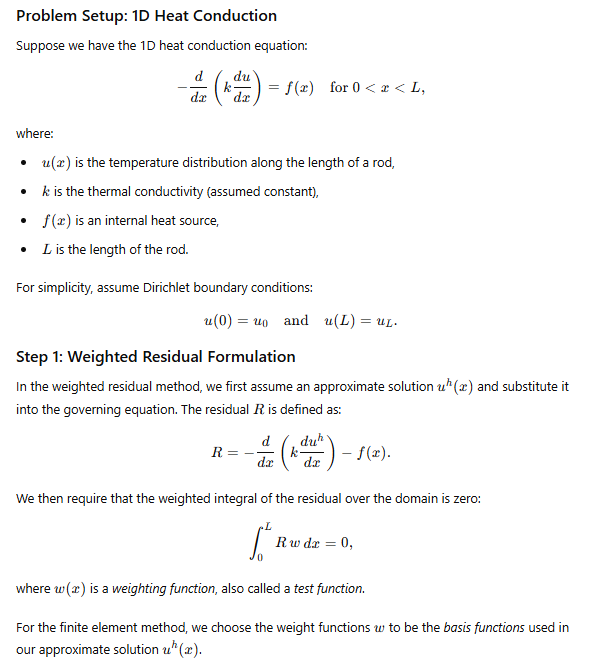
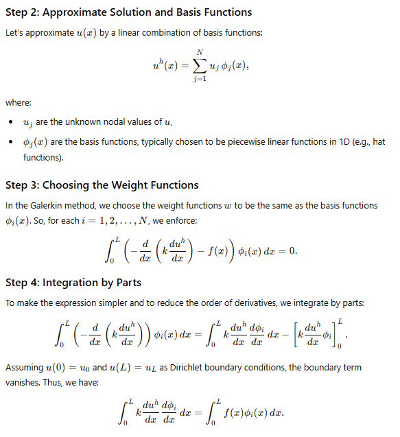
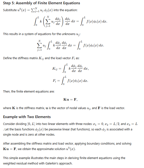
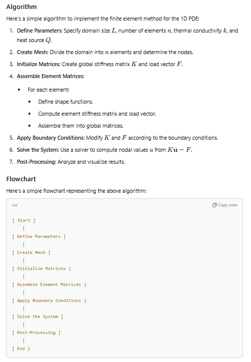
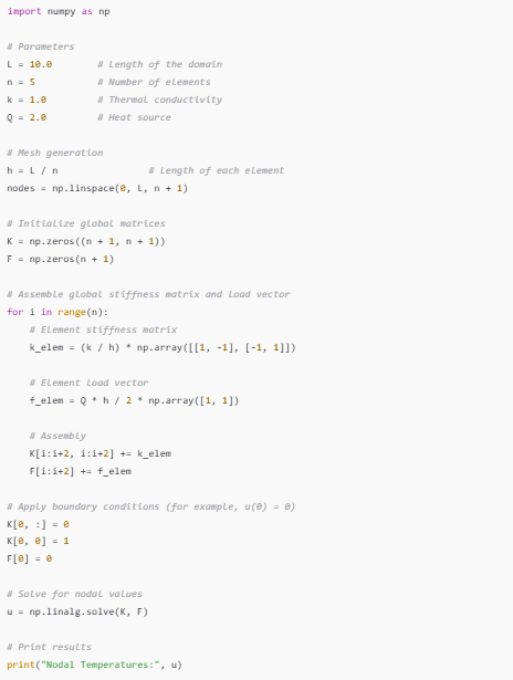
Pada tugas 1 Komputasi Teknik kami diarahkan oleh Pak DAI untuk melakukan diskusi dengan menggunakan ChatGPT mengenai finite element equation dari 1D PDE yang diselaraskan dengan DAI5 Framework. Berikut merupakan hasil diskusi saya dengan ChatGPT.
User Question :
Can you derive finite element equations from 1D PDE governing equations using weighted residual in a very simple way along with an example.
ChatGPT Answer :
User Question :
Can you provide with algorithm, flow chart and python code.
ChatGPT Answer :
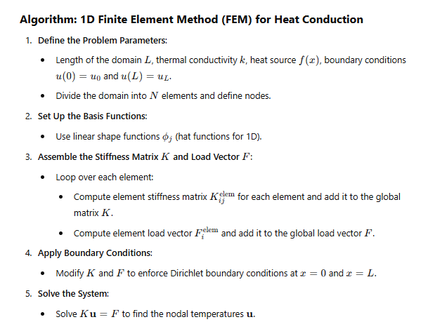
Algorithm
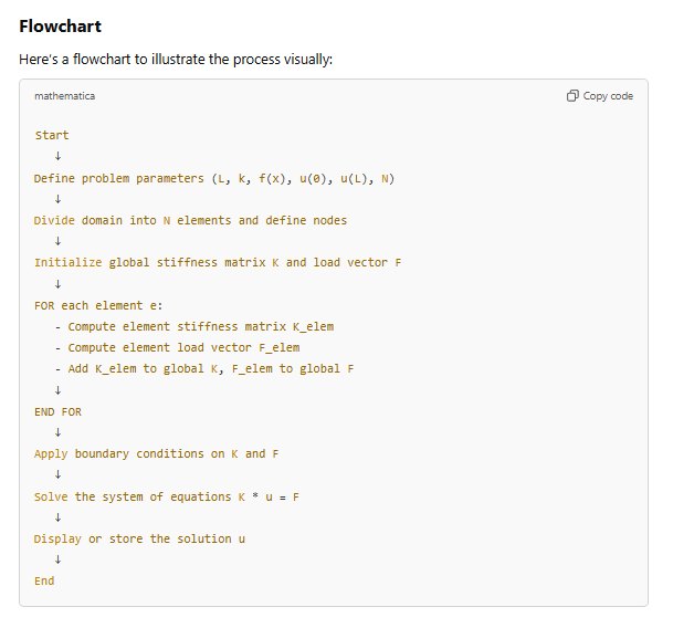
Flow Chart
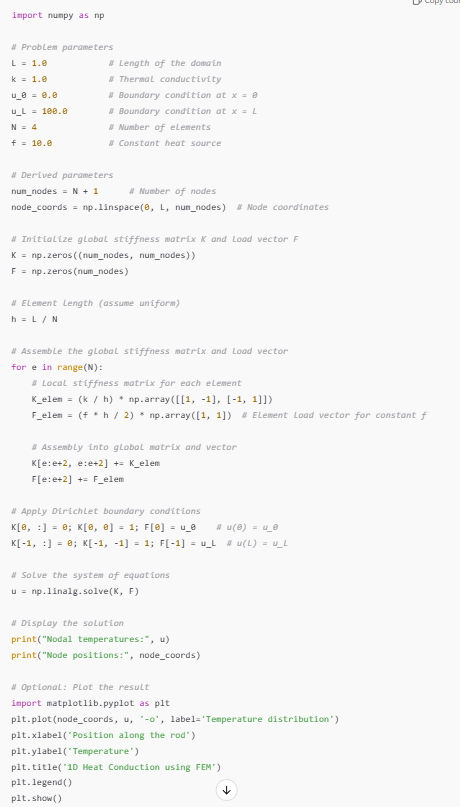
Python Code
User Question :
Can you restructure all of your above explanation using DAI5 Framework with intention step as fundamental step as you also mentioned in the following : Free will naturally ties into the DAI5 framework because both free will and consciousness play vital roles in the intention-setting and decision-making processes that drive each step in DAI5. With conscious intention as a central element in DAI5, free will could be seen as the "engine" that enables individuals to choose how to direct that consciousness. This conscious choice—the exercise of free will—could then influence each step, from problem understanding to creating solutions that align with one’s ultimate goals.
ChatGPT Answer :
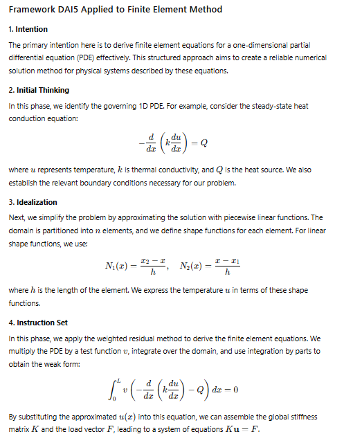
DAI5 Framework Application
Algorithm and Flow Chart
Python Code
Conclusion
Dengan menerapkan kerangka kerja DAI5 pada penurunan persamaan elemen hingga, dapat dilakukan dengan mempertahankan pendekatan terstruktur selama proses berlangsung. Setiap langkah-mulai dari menetapkan tujuan hingga memahami masalah, menyederhanakannya, dan merumuskan langkah-langkah yang dapat ditindaklanjuti-memastikan hasil yang akurat dan bermakna. Metode ini menekankan pengambilan keputusan secara sadar dan pertimbangan etis dalam proses analisis teknik.
Pertemuan 2 - Komputasi Teknik (5 November 2024)
Pada pertemuan kedua Pak DAI menginstruksikan kepada mahasiswa untuk mencari perbedaan dalam pengetahuan dan pola pikir mahasiswa teknik mesin antara mahasiswa S1, S2, dan S3. Dalam menjawab persoalan tersebut Pak DAI mengarahkan agar pencarian dibantu menggunakan ChatGPT. Adapun hasil dari diskusi dengan ChatGPT sebagai berikut ini.
User Question : Give me a question, the question is in three level of degree. One for an undergraduate student, two for a magister student, and three for doctoral student. The question context must be related to mechanical engineering.
ChatGPT Answer :
Undergraduate Level (Basic Understanding) Question: Explain the principles of the first law of thermodynamics and describe how it applies to a closed system. Provide an example of a closed system in everyday life where energy conservation plays a significant role.
Magister Level (Advanced Application) Question: Analyze the effects of thermal conductivity, convection, and radiation in the heat transfer process for an insulated pipeline transporting hot fluid. How would you optimize the insulation to minimize energy loss while considering material and operational costs?
Doctoral Level (Research-Oriented Challenge) Question: Develop a theoretical model to predict heat transfer and energy loss in a multi-layered composite material system used in high-temperature industrial applications. How would you incorporate material heterogeneity and thermal stress factors into your model, and what numerical methods would you use to validate it against experimental data?
User Question : What is the main difference between thee question given above?
ChatGPT Answer :
The main differences between the questions at each academic level lie in depth of understanding, complexity of analysis, and scope of application:
1. Depth of Understanding:
Undergraduate Level: The question focuses on foundational principles, expecting a basic understanding of concepts like energy conservation within a closed system. It doesn’t require detailed technical calculations or modeling, only a conceptual explanation with an everyday example. Magister Level: The question requires a deeper understanding and practical application of heat transfer modes (conduction, convection, radiation). Here, students need to analyze specific engineering problems, consider optimization, and balance cost with effectiveness, demonstrating a more technical grasp. Doctoral Level: The doctoral question expects an advanced theoretical understanding and research-level approach, asking students to build a predictive model. They must consider complexities like material heterogeneity and thermal stresses, pushing beyond established principles to create and validate new methodologies.
2. Complexity of Analysis:
Undergraduate Level: Analysis is relatively simple, mainly focused on explaining core principles and basic applications. Magister Level: Analysis becomes more complex, involving multi-mode heat transfer, cost considerations, and practical engineering trade-offs. Doctoral Level: Analysis is the most complex, involving theoretical modeling, advanced computational methods, and validation through experimental data. This requires not just understanding of principles but also innovation in approach and tools.
3. Scope of Application:
Undergraduate Level: The application is broad and general, aimed at helping students recognize thermodynamics concepts in everyday scenarios. Magister Level: Application focuses on a specific, practical engineering system (e.g., an insulated pipeline) where students must apply advanced knowledge to optimize real-world solutions. Doctoral Level: Application is research-oriented, dealing with new or less understood systems. Here, students contribute to advancing the field by developing models that can be validated and applied in high-precision or high-stakes industrial settings.
Pada kelas Pak DAI menginstruksikan kami untuk diberikan jawaban mengenai one dimension heat conduction untuk mengetest pemahaman kami pada topik yang sedang dibahas tersebut. Didapatkan hasil sebagai berikut :
User Question : Please give me 5 questions about 1 dimension heat conduction. Can you give me in multiple choice and in Bahasa. Don't give me the answer, i will anser it myself, and then you can assess my answer.
ChatGPT Answer :
1. Apa hukum dasar yang digunakan untuk mendeskripsikan aliran panas dalam konduksi satu dimensi?
A. Hukum Newton B. Hukum Stefan-Boltzmann C. Hukum Fourier D. Hukum Avogadro
2. Pada konduksi panas satu dimensi dalam kondisi tunak, bagaimana perubahan suhu terhadap waktu?
A. Suhu meningkat seiring waktu B. Suhu berkurang seiring waktu C. Suhu tidak berubah seiring waktu D. Suhu berubah secara periodik seiring waktu
3. Kondisi batas tipe Dirichlet pada masalah konduksi panas satu dimensi menyatakan bahwa:
A. Suhu di ujung batang ditentukan secara tetap B. Fluks panas di ujung batang adalah konstan C. Fluks panas di ujung batang adalah nol D. Konduktivitas termal di ujung batang beragam
4. Apa keuntungan utama dari metode elemen hingga (finite element method) dalam memecahkan masalah konduksi panas satu dimensi?
A. Dapat memecahkan masalah dengan variabel dan geometri kompleks B. Memastikan hasilnya selalu tepat C. Membutuhkan sedikit data untuk pemecahan masalah D. Lebih cepat dibandingkan metode eksperimental
5. Bagaimana pengaruh konduktivitas termal k suatu material terhadap distribusi suhu dalam batang satu dimensi yang mengalami aliran panas?
A. Semakin tinggi konduktivitas termal, semakin besar gradien suhu B. Semakin rendah konduktivitas termal, semakin kecil gradien suhu C. Semakin tinggi konduktivitas termal, semakin kecil gradien suhu D. Konduktivitas termal tidak mempengaruhi distribusi suhu
Hasil akhir dari penilaian saya adalah sebagai berikut :
Berikut adalah penilaian berdasarkan jawaban Anda: Benar (C. Hukum Fourier) Benar (C. Suhu tidak berubah seiring waktu) Benar (A. Suhu di ujung batang ditentukan secara tetap) Benar (A. Dapat memecahkan masalah dengan variabel dan geometri kompleks) Salah (Jawaban yang benar: C. Semakin tinggi konduktivitas termal, semakin kecil gradien suhu) Skor Anda: 4 dari 5. Anda memperoleh 80%. Bagus sekali!
Tugas 2 - Komputasi Teknik
Tugas : Lakukan penyelesaian permasalahan 1D finite element dalam heat transfer dengan menggunakan pendekatan conscious continuum dan framework DAI 5, buatkan ke dalam aplikasi Python dalam menentukan kondisi pemanasan pada pipa.
Penjelasan Conscious Continuum Menurut ChatGPT
The term "conscious continuum" suggests a concept where continuity is viewed through a lens of awareness and intentionality, especially in the context of problem-solving or scientific analysis. It merges the technical idea of continuity from fields like continuum mechanics with a perspective that emphasizes conscious awareness and purpose at every step of an analysis or process.
Here’s how conscious continuum can apply in different contexts:
1. In Engineering and Physics (Continuum Mechanics): A material is often treated as continuous, assuming no breaks or discontinuities at the microscopic scale. By adding "conscious" to this concept, one might approach each step in the analysis with a clear, deliberate awareness of how small-scale phenomena contribute to the larger, smooth continuum. This means not only treating the material as continuous but doing so with a focused understanding of the process's holistic goal.
2. In Problem Solving (Frameworks like DAI5): A conscious continuum can imply an approach where each stage of analysis—from intention to execution—is approached with mindfulness and deliberate purpose. This continuity of conscious focus across each phase can help in achieving solutions that align with both technical accuracy and broader values, like sustainability or ethical responsibility.
Diskusi Terkait Conscious Continuum dan kaitannya dengan DAI5 Framework
User Question : Can you give a practical example (along with simple calculator such as 1D Problem) ,In engineering that continuum mechanics treatsmaterials as continuous, on integration of uninterrupted "conscious continuum" into the DAI5 framework.
ChatGPT Answer :
To practically apply a continuum mechanics approach integrated with the DAI5 framework in an engineering context, let’s explore a 1D heat conduction problem within a continuum material, for example, a metal rod. This scenario illustrates how material properties can be seen as continuous along the rod, with temperature changes occurring smoothly across its length. Here, we’ll follow each step of the DAI5 framework with a conscious integration approach to illustrate the problem's analysis and solution.
Problem Setup Let’s consider a metal rod of length 𝐿=1𝑚, fixed at one end at temperature 𝑇=100∘C and the other end at 𝑇=0∘C. The goal is to determine the temperature distribution along the rod in steady state, assuming no heat generation within the material (using the 1D steady-state heat conduction equation).
The differential equation governing this process is:
(...)
This equation represents the continuum treatment, assuming temperature changes without any abrupt jumps or gaps across the rod.
Applying the DAI5 Framework with Conscious Continuum Integration
1). Intention
Set a clear intention to solve the temperature distribution problem with an awareness of the material's continuous nature. Here, we aim not only to find a solution but to ensure it reflects the rod's physical behavior as a continuous entity, emphasizing stability and accuracy.
2). Initial Thinking
Develop an understanding of the physical laws and principles underlying heat conduction. In this case, Fourier’s law applies, assuming a homogenous material where thermal conductivity 𝑘 is constant. Recognizing the boundary conditions helps define the continuum’s extent: a fixed temperature at both ends ensures a steady-state solution across the rod.
3). Idealization
Simplify the problem by assuming: - The rod is perfectly insulated along its length, so there is no heat loss to the surroundings. - Material properties like thermal conductivity remain constant, reflecting an uninterrupted “conscious continuum” across the rod's length. This idealization provides a manageable framework while maintaining accuracy.
4). Instruction Set
Using the finite element method (FEM), break down the rod into discrete elements (nodes) while treating the material properties as continuous between nodes. Here, we will calculate the temperature distribution at different points along the rod.
The discretized version of the governing equation becomes:
(...)
This is solved with Dirichlet boundary conditions: T(0)=100 and T(L)=0
5). Instruction Set and Python Code Example
import numpy as np import matplotlib.pyplot as plt
- Problem setup
L = 1.0 # Length of the rod in meters N = 10 # Number of elements T0, TL = 100, 0 # Boundary temperatures k = 1 # Thermal conductivity (constant)
- Discretize the domain
x = np.linspace(0, L, N+1) # N+1 nodes dx = L / N # Element length
- Initialize temperature array
T = np.zeros(N+1) T[0] = T0 # Set boundary at x=0 T[-1] = TL # Set boundary at x=L
- Build and solve the linear system
A = np.zeros((N+1, N+1)) # Coefficient matrix b = np.zeros(N+1) # Right-hand side vector
- Fill the matrix A and vector b
for i in range(1, N):
   A[i, i-1] = A[i, i+1] = k / dx**2
   A[i, i] = -2 * k / dx**2
b[0], b[-1] = T0, TL
- Apply boundary conditions
A[0, 0] = A[-1, -1] = 1 A[0, 1] = A[-1, -2] = 0
- Solve the system
T = np.linalg.solve(A, b)
- Plot the result
plt.plot(x, T, '-o', label="Temperature Distribution") plt.xlabel("Position along the rod (m)") plt.ylabel("Temperature (°C)") plt.title("1D Heat Conduction in a Rod") plt.legend() plt.grid(True) plt.show()
Hasil Codingan Grafik
(...)
Pertanyaan Hasil Diskusi
User Question : can you explain to me the recent answer you gave me about "a practical example (along with simple calculator such as 1D Problem) ,In engineering that continuum mechanics treatsmaterials as continuous, on integration of uninterrupted "conscious continuum" into the DAI5 framework". Tell why is the governing equation is like you mentioned before, give me a comprehensive answer about why is the discretized version of the governing equation becomes like you mentioned in the answer, and what is the meaning of "solved with Dirichlet boundary conditions", and please explain to me about the python code you made for the example because i don't really get what is you trying to do. Please explain to me why you use matrix in this example?
ChatGPT Answer :
Problem Setup: 1D Heat Conduction
We are solving a 1D steady-state heat conduction problem for a rod of length 𝐿, with known temperatures at both ends. This setup means that heat flows along the rod but does not change over time (steady state).
1). Governing Equation
In 1D steady-state heat conduction without any internal heat generation, the temperature distribution 𝑇(𝑥) along the rod satisfies the heat conduction (Poisson) equation:
(...)
This equation comes from Fourier's law of heat conduction, which states that the heat flux 𝑞 is proportional to the temperature gradient dT/dx. In steady state, the heat flux does not vary along the rod (no sources or sinks inside the rod), which simplifies the equation to a second derivative of 𝑇(𝑥) equal to zero.
2). Discretized Version of the Governing Equation
To solve this equation numerically, we discretize the domain by dividing the rod into 𝑁 segments. Each segment is represented by nodes (points along the rod), and we use these nodes to approximate the temperature at each position.
(...)
3). Dirichlet Boundary Conditions
Boundary conditions are necessary to solve the differential equation. Here, we use Dirichlet boundary conditions, meaning that the temperature is fixed at both ends of the rod:
(...)
These boundary conditions specify the exact temperatures at the boundaries, allowing us to compute the temperature distribution along the rod between these two endpoints.
4). Explanation of the Python Code
import numpy as np import matplotlib.pyplot as plt
- Problem setup
L = 1.0 # Length of the rod in meters N = 10 # Number of elements T0, TL = 100, 0 # Boundary temperatures k = 1 # Thermal conductivity (constant)
Explanation :
We set the length 𝐿 of the rod to 1 meter and specify 𝑁=10 segments, meaning the rod will have 𝑁+1 nodes (points of calculation). T0 and 𝑇𝐿 represent the fixed temperatures (boundary conditions) at each end of the rod. 𝑘 is the thermal conductivity, assumed to be constant here.
- Discretize the domain
x = np.linspace(0, L, N+1) # N+1 nodes dx = L / N # Element length
Explanation
We divide the rod into 𝑁 elements, generating 𝑁+1 points along the rod using np.linspace(0, L, N+1). This gives the locations (positions) of the nodes. 𝑑𝑥 is the spacing between nodes (element length).
- Initialize temperature array
T = np.zeros(N+1) T[0] = T0 # Set boundary at x=0 T[-1] = TL # Set boundary at x=L
Explanation
We initialize an array T to store the temperature at each node. The temperature at the first (T[0]) and last (T[-1]) nodes is set to the boundary values 𝑇0 and 𝑇𝐿, respectively.
- Build and solve the linear system
A = np.zeros((N+1, N+1)) # Coefficient matrix b = np.zeros(N+1) # Right-hand side vector
- Fill the matrix A and vector b
for i in range(1, N):
   A[i, i-1] = A[i, i+1] = k / dx**2
   A[i, i] = -2 * k / dx**2
b[0], b[-1] = T0, TL
Explanation
(...)
A[0, 0] = A[-1, -1] = 1 A[0, 1] = A[-1, -2] = 0
Explanation These lines enforce the boundary conditions. A[0,0] = 1 and A[-1,-1] = 1 set the first and last entries to match the boundary temperatures exactly. We ensure the temperature at these nodes doesn’t change, reflecting the Dirichlet conditions.
- Solve the system
T = np.linalg.solve(A, b)
Explanation
The np.linalg.solve(A, b) function solves the linear system to obtain the temperature T at each node.
- Plot the result
plt.plot(x, T, '-o', label="Temperature Distribution") plt.xlabel("Position along the rod (m)") plt.ylabel("Temperature (°C)") plt.title("1D Heat Conduction in a Rod") plt.legend() plt.grid(True) plt.show()
Explanation
This part of the code plots the temperature distribution along the rod, with x as the position and T as the temperature at each position.
5). Matrix Representation of the Finite Difference Equations
When we discretize the continuous 1D heat conduction equation, we approximate the temperature at each node by applying finite difference methods. For an internal node 𝑖, we have:
(...)
This equation relates the temperatures at adjacent nodes. Repeating this process for each internal node leads to a system of equations where each equation connects several temperatures.
This system can be rewritten in the form: A.T=b,
(...)
Using matrices allows us to compactly represent this large system of equations. In matrix form:
-Each row in 𝐴 represents one of the finite difference equations. -The diagonal and off-diagonal entries in 𝐴 correspond to the coefficients of 𝑇𝑖 and its neighboring nodes, capturing the relationships between the nodes in one structure.
When we use matrices, we can solve for the unknowns in a highly systematic way. In our example:
𝑇, the vector of unknown temperatures, is calculated using 𝑇=𝐴^−1.𝑏, or more efficiently with a direct solver like np.linalg.solve(A, b). By using a matrix structure, we leverage linear algebra techniques that are efficient and reliable for solving such systems.
Applying boundary conditions directly to a matrix system is straightforward and organized. For example:
By setting rows in 𝐴 to enforce the boundary conditions, we fix values at the endpoints without needing additional adjustments in the solution.
