Difference between revisions of "Thareq Wibisono"
| Line 15: | Line 15: | ||
Last session of the class we are given a task to learn the open-modelica software as to get the general workflow of the software and its feeling. The main learning source for my learning journey is via youtube and a website titled "Modelica by Example" created by Dr. Michael M. Tiller. I began my journey with the familiarity of modelica language which is the driving program for the software. The syntax of the program, like most of the available high-language program, contain a familiar properties such as the if, elif, and else statement, iteration with for and while loop, variable declaration, array, etc. I tried to play around with the language and manage to write several interesting program. One of those is a function that return a calculation of a polynomial algebaric expression. The script is shown below | Last session of the class we are given a task to learn the open-modelica software as to get the general workflow of the software and its feeling. The main learning source for my learning journey is via youtube and a website titled "Modelica by Example" created by Dr. Michael M. Tiller. I began my journey with the familiarity of modelica language which is the driving program for the software. The syntax of the program, like most of the available high-language program, contain a familiar properties such as the if, elif, and else statement, iteration with for and while loop, variable declaration, array, etc. I tried to play around with the language and manage to write several interesting program. One of those is a function that return a calculation of a polynomial algebaric expression. The script is shown below | ||
| − | [[File:Polynomial evaluator.PNG]] | + | [[File:Polynomial evaluator.PNG|800px|thumb|center|'''Figure 2.''' Code script for polynomial evaluator function]] |
As you can see form the script, the function takes x as the input and return fx as the output. The parameter (variable that remain constant through out the simulation) is written below the protected statement which include the polynomial constant a, b, and c. Because we are dealing with the Real number, we must specified it after typing the parameter. The algorithm statement will carry out the actual evaluation which in this case will return fx as the output | As you can see form the script, the function takes x as the input and return fx as the output. The parameter (variable that remain constant through out the simulation) is written below the protected statement which include the polynomial constant a, b, and c. Because we are dealing with the Real number, we must specified it after typing the parameter. The algorithm statement will carry out the actual evaluation which in this case will return fx as the output | ||
| Line 21: | Line 21: | ||
Because it is a function, it cannot be simulated directly. So I create a new class, which are able to call and simulate the function, with the following script | Because it is a function, it cannot be simulated directly. So I create a new class, which are able to call and simulate the function, with the following script | ||
| − | [[File:Polynomial checker.PNG]] | + | [[File:Polynomial checker.PNG|800px|thumb|center|'''Figure 3.''' Code script for simulating polynomial evaluator]] |
which will return the following result | which will return the following result | ||
| − | [[File:Result polyEval.PNG]] | + | [[File:Result polyEval.PNG|800px|thumb|center|'''Figure 4.''' Result for polynomial evaluator function]] |
Another program that I write is the bouncing ball program which calculate the bouncing trajectory of a free falling ball when hitting the ground. The script to the program is shown below | Another program that I write is the bouncing ball program which calculate the bouncing trajectory of a free falling ball when hitting the ground. The script to the program is shown below | ||
| − | [[File:Bouncing ball.PNG]] | + | [[File:Bouncing ball.PNG|800px|thumb|center|'''Figure 5.''' Code script for simulating the trajectory of a bouncing ball]] |
In short the program will try to calculate the trajectory and the velocity of the ball. When the ball is bounced back, the velocity is decrease by a constant e. When the ball reach 0 m in height, the program will terminate. The resulting plot is shown below | In short the program will try to calculate the trajectory and the velocity of the ball. When the ball is bounced back, the velocity is decrease by a constant e. When the ball reach 0 m in height, the program will terminate. The resulting plot is shown below | ||
[[File:Bouching ball result.png]] | [[File:Bouching ball result.png]] | ||
Revision as of 09:06, 3 March 2021
Date: 23 Feb 2021
Today I have learn about the correlation between justice and its usage in our current mechanical knowledge. Although it is rather an odd correlation as justice refers to the socio-economic term, the meaning of justice itself express the state of equilibrium in which one does not have to do another work to balance out the inequalities. As an engineer, justice is important not only to uphold social inequalities but also, in a more technical sense, an obligatory to understand how physical system works through a mathematical equations. Any physical system will find its own way to reach a state of equilibrium by increasing its entropy. By the time it reach the state of equilibrium, the entropy will reach its maximum level and any entities within the mathematical equation will balanced out.
But before dwell deeper to the topic, a simple definition to energy must be provided as many still have a vague idea about the term. The energy can be explained as the ability to do work, as one of my classmate says. It is a mechanism that structured life. like the flowing water, the energy is not stagnant. It constantly deliver one self to another entities in a various form. For example when we do an activity, we tend to be in exhaustion state by running a few kilometers as the energy is flowing from the chemical energy in our body to mechanical energy by moving our leg and dissipated as heat to the environment.
Date: 24 Feb 2021
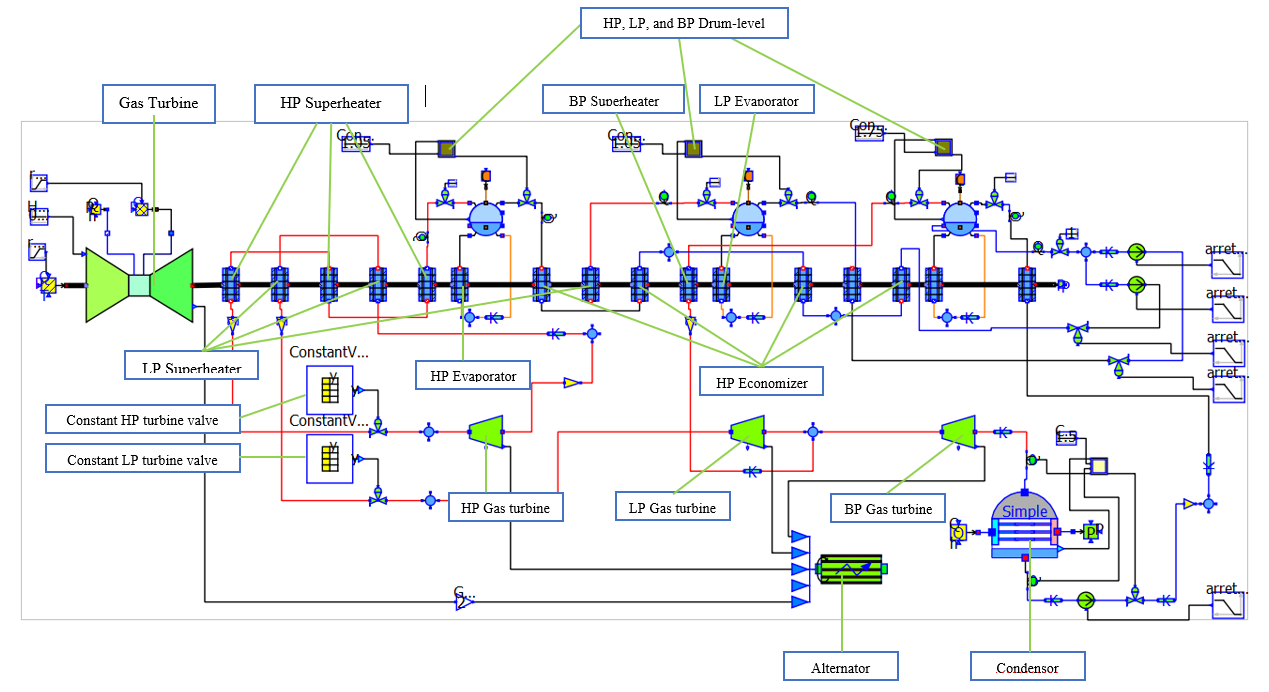
The assignment given yesterday is to define the component of the combined cycle plant which are shown below
Date: 2 March 2021
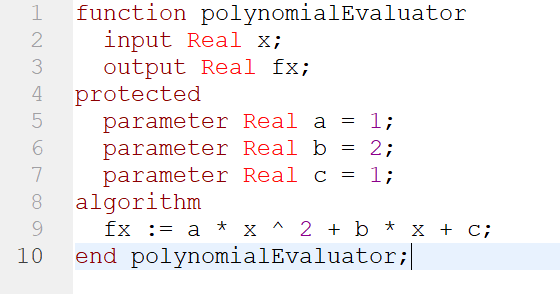
Last session of the class we are given a task to learn the open-modelica software as to get the general workflow of the software and its feeling. The main learning source for my learning journey is via youtube and a website titled "Modelica by Example" created by Dr. Michael M. Tiller. I began my journey with the familiarity of modelica language which is the driving program for the software. The syntax of the program, like most of the available high-language program, contain a familiar properties such as the if, elif, and else statement, iteration with for and while loop, variable declaration, array, etc. I tried to play around with the language and manage to write several interesting program. One of those is a function that return a calculation of a polynomial algebaric expression. The script is shown below
As you can see form the script, the function takes x as the input and return fx as the output. The parameter (variable that remain constant through out the simulation) is written below the protected statement which include the polynomial constant a, b, and c. Because we are dealing with the Real number, we must specified it after typing the parameter. The algorithm statement will carry out the actual evaluation which in this case will return fx as the output
Because it is a function, it cannot be simulated directly. So I create a new class, which are able to call and simulate the function, with the following script
which will return the following result
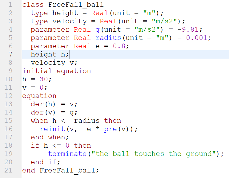
Another program that I write is the bouncing ball program which calculate the bouncing trajectory of a free falling ball when hitting the ground. The script to the program is shown below
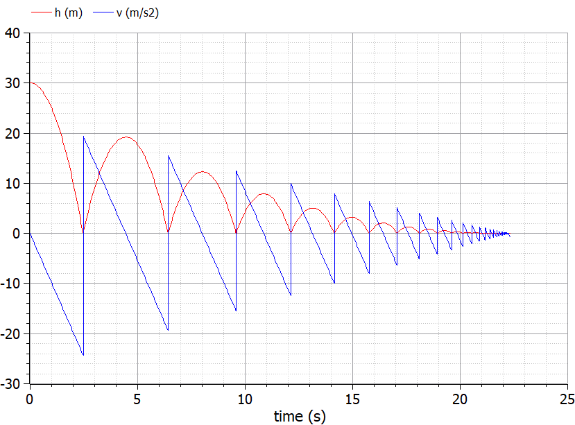
In short the program will try to calculate the trajectory and the velocity of the ball. When the ball is bounced back, the velocity is decrease by a constant e. When the ball reach 0 m in height, the program will terminate. The resulting plot is shown below


