Difference between revisions of "Izzuddin Al Qossam"
Izzuddin.aq (talk | contribs) |
Izzuddin.aq (talk | contribs) (→2.4.2. Properties) |
||
| (241 intermediate revisions by the same user not shown) | |||
| Line 1: | Line 1: | ||
| − | '''Background''' | + | Halo, Assalamu'alaikum Warahmatullahi Wabarakatuh, perkenalkan nama saya Izzuddin Al Qossam, mahasiswa S2 Teknik Mesin Universitas Indonesia dengan Nomor Pokok Mahasiswa (NPM): 2206131684 |
| + | |||
| + | |||
| + | __TOC__ | ||
| + | |||
| + | |||
| + | |||
| + | |||
| + | == '''Background''' == | ||
| + | |||
Penelitian saya terkait steam combustion pada incinerator MSW. Kegiatan ini merupakan kolaborasi antara Laboratorium Gasifikasi dan PT Bumiresik Nusantara Raya. Permasalahan yang ingin diselesaikan adalah bagaimana asap pembakaran sampah pada incinerator menjadi lebih bersih dan tidak terjadi overheated. Salah satu inovasi yang coba dikembangkan adalah intermittent furnace dengang dual chamber. Primary chamber menggunakan sistem superheated steam untuk meningkatkan suhu pembakaran sampah dengan jumlah yang sampah yang lebih sedikit. Secondary chamber digunakan untuk pembakaran sampah dengan volume sampah lebih banyak dan terhubung dengan primary chamber. Tujuan adanya intermittent furnace agar efek dari steam combustion dapat meningkatkan pembakaran pada secondary chamber dan mencegah adanya overheated pada secondary chamber. | Penelitian saya terkait steam combustion pada incinerator MSW. Kegiatan ini merupakan kolaborasi antara Laboratorium Gasifikasi dan PT Bumiresik Nusantara Raya. Permasalahan yang ingin diselesaikan adalah bagaimana asap pembakaran sampah pada incinerator menjadi lebih bersih dan tidak terjadi overheated. Salah satu inovasi yang coba dikembangkan adalah intermittent furnace dengang dual chamber. Primary chamber menggunakan sistem superheated steam untuk meningkatkan suhu pembakaran sampah dengan jumlah yang sampah yang lebih sedikit. Secondary chamber digunakan untuk pembakaran sampah dengan volume sampah lebih banyak dan terhubung dengan primary chamber. Tujuan adanya intermittent furnace agar efek dari steam combustion dapat meningkatkan pembakaran pada secondary chamber dan mencegah adanya overheated pada secondary chamber. | ||
| Line 5: | Line 14: | ||
Langkah awal penelitian dilakukan dengan pemodelan ASPEN Plus dan CFD agar dapat melihat karakteristik steam pada pembakaran dan karakteristik distribusi temperatur pada furnace. | Langkah awal penelitian dilakukan dengan pemodelan ASPEN Plus dan CFD agar dapat melihat karakteristik steam pada pembakaran dan karakteristik distribusi temperatur pada furnace. | ||
| − | Saya menggunakan DAI5 Conscious Thinking Framework sebagai landasan berpikir untuk menyelesaikan masalah di pengaplikasian CFD. [[https://www. | + | ---- |
| + | |||
| + | |||
| + | |||
| + | |||
| + | == '''DAI5 Conscious Thinking Framework''' == | ||
| + | |||
| + | |||
| + | Framework DAI5 adalah pendekatan penyelesaian masalah yang baru dan menekankan metode yang komprehensif, terstruktur, serta melibatkan kesadaran penuh. DAI5 merupakan singkatan dari '''Dr. Ahmad Indra''' sebagai pencipta dan pengembang framework ini dan empat tahapan utama: '''Intention''' (Niat), '''Initial Thinking''' (Pemikiran Awal), '''Idealization''' (Idealisasi), dan '''Instruction Set''' (Set Instruksi). | ||
| + | |||
| + | '''1. Dr. Ahmad Indra:''' Nama ini mengacu pada pencipta dan pengembang framework DAI5, yaitu Dr. Ahmad Indra. Framework ini dikembangkan dengan latar belakang filosofi dan pendekatan khusus yang dirumuskan oleh beliau dalam upaya untuk menciptakan solusi problem solving berbasis conscious thinking. | ||
| + | |||
| + | '''2. ''Intention'' (Niat):''' Langkah awal yang mengarahkan seluruh proses penyelesaian masalah. Dalam tahap ini, niat dan tujuan yang jelas harus ditentukan, dan sering kali niat tersebut mengandung elemen spiritual yang berhubungan dengan usaha untuk mencari ridho Tuhan. Subjektivitas sangat mempengaruhi niat, yang dapat bervariasi tergantung pada pengalaman pribadi, nilai, dan keyakinan individu. | ||
| + | |||
| + | '''3. ''Initial Thinking'' (Pemikiran Awal):''' Ini adalah tahapan di mana dilakukan eksplorasi awal terhadap masalah, yang meliputi pengumpulan informasi dan pemahaman yang lebih mendalam tentang konteks permasalahan. Tahap ini melibatkan analisis awal untuk mendapatkan gambaran besar serta prinsip-prinsip dasar yang terlibat dalam permasalahan. | ||
| + | |||
| + | '''4. ''Idealization'' (Idealisasi):''' Pada tahap ini, masalah yang kompleks disederhanakan melalui berbagai asumsi atau pendekatan yang dapat dipertanggungjawabkan. Tujuannya adalah untuk memfokuskan hanya pada variabel-variabel penting sehingga masalah menjadi lebih terarah dan mudah diselesaikan. | ||
| + | |||
| + | '''5. ''Instruction Set'' (Set Instruksi):''' Tahap terakhir di mana langkah-langkah terstruktur dan sistematis disusun untuk menyelesaikan masalah. Ini berfungsi sebagai panduan yang jelas, berdasarkan hasil dari proses idealisasi sebelumnya. | ||
| + | |||
| + | Framework DAI5 ini menekankan kesadaran penuh dalam setiap tahap penyelesaian masalah, yang membedakannya dari metode lain yang lebih teknis dan objektif, karena ia juga mempertimbangkan aspek spiritual dan subjektivitas pribadi. Saya menggunakan DAI5 Conscious Thinking Framework ini sebagai landasan berpikir untuk menyelesaikan masalah di pengaplikasian CFD. | ||
| + | |||
| + | |||
| + | <youtube width="200" height="100">JpTDnFLc2Yk </youtube> | ||
| + | |||
| + | |||
| + | ---- | ||
| + | |||
| + | |||
| + | |||
| + | |||
| + | == '''Aplikasi CFD pada Lid Driven Cavity Flow''' == | ||
| + | |||
| + | |||
| + | |||
| + | === '''1. Pembentukan Vorteks Primer:''' === | ||
| + | |||
| + | |||
| + | Vorteks primer terbentuk sebagai pola aliran sirkular dominan yang disebabkan oleh pergerakan tutup (lid driven cavity). Ketika tutup bergerak secara tangensial, ia menyeret fluida yang ada di dekatnya, menghasilkan gaya gesekan yang menyebabkan fluida berputar di dalam rongga. Ini menciptakan aliran sirkulasi yang dikenal sebagai vorteks primer, yang memusat di sekitar bagian tengah rongga. Vorteks primer biasanya berada di pusat rongga dan berbentuk elips atau lingkaran, bergantung pada bilangan Reynolds dan aspek rasio rongga. | ||
| + | |||
| + | |||
| + | === '''2. Pembentukan Vorteks Sekunder:''' === | ||
| + | |||
| + | |||
| + | Vorteks sekunder terbentuk di dekat dinding-dinding yang stasioner, terutama di sudut-sudut rongga. Vorteks ini lebih kecil dan kurang kuat dibandingkan vorteks primer. Vorteks sekunder terjadi karena aliran fluida di sudut-sudut tersebut terjebak oleh aliran sirkulasi vorteks primer, sehingga terbentuk pola sirkulasi lokal di area sudut tersebut. Vorteks sekunder terbentuk di sudut kiri bawah dan kanan bawah rongga, serta kadang-kadang di sudut atas, tergantung pada kondisi aliran. Pada bilangan Reynolds yang rendah (aliran laminar), vorteks sekunder berukuran kecil dan lemah, namun seiring dengan meningkatnya bilangan Reynolds, vorteks sekunder menjadi lebih besar dan lebih jelas. Bahkan, pada aliran turbulen yang lebih tinggi, vorteks tersier bisa muncul di beberapa sudut. | ||
| + | |||
| + | [[File:Reynold numbers.png|1200px]] | ||
| + | |||
| + | |||
| + | |||
| + | === '''Dinamika Vorteks dan Bilangan Reynolds:''' === | ||
| + | |||
| + | |||
| + | '''-> Pada Bilangan Reynolds Rendah (aliran laminar):''' Vorteks primer mendominasi, sementara vorteks sekunder lemah dan terbatas di sudut-sudut rongga. Aliran cenderung halus dan teratur. | ||
| + | |||
| + | '''-> Pada Bilangan Reynolds Tinggi (aliran transisional dan turbulen):''' Vorteks primer mulai terdeformasi, dan vorteks sekunder serta tersier dapat muncul karena ketidakstabilan aliran yang lebih besar. | ||
| + | |||
| + | Pembentukan vorteks primer dan sekunder ini merupakan hasil dari interaksi antara tutup yang bergerak, dinding yang diam, dan gaya viskos pada fluida. Fenomena ini sering dipelajari dengan menggunakan metode numerik seperti metode beda hingga atau simulasi lattice-Boltzmann untuk menyelesaikan persamaan Navier-Stokes yang mendeskripsikan aliran fluida | ||
| + | |||
| + | Berikut analisis saya terhadap aliran pada Lid Driven Cavity menggunakan aplikasi OpenFoam dengan variasi dynamic viscosity untuk mengetahui profil aliran. | ||
| + | |||
| + | |||
| + | <youtube width="200" height="100">4QMIz-k7Js0 </youtube> | ||
| + | |||
| + | |||
| + | Referensi hasil analisis aliran didapatkan dari jurnal '''''"The Lid-Driven Cavity"''''' dengan penulis ''Hendrik C. Kuhlmann'' dan ''Francesco Romanò''. Berikut adalah rangkuman jurnalnya. [https://docs.google.com/presentation/d/1DRwm_AR6CxAWdLzqvewv-IvehVmvEJB5/edit?usp=sharing&ouid=103849052379933915869&rtpof=true&sd=true] | ||
| + | |||
| + | ---- | ||
| + | |||
| + | == '''Self-Assesment using Chat-GPT''' == | ||
| + | |||
| + | |||
| + | '''I used Chat-GPT not Cheat-GPT for Self-Assessment Mid-Test of Computational Fluid Dynamics''' | ||
| + | |||
| + | You can read my interactions with Chat-GPT by clicking this link [https://chatgpt.com/share/671af6fb-dfac-8003-b5ff-6df5140cee28] | ||
| + | |||
| + | |||
| + | |||
| + | === '''Basic CFD Test''' === | ||
| + | |||
| + | |||
| + | '''1. What does CFD stand for?''' | ||
| + | |||
| + | a) Computational Fluid Dynamics | ||
| + | |||
| + | b) Complex Fluid Dynamics | ||
| + | |||
| + | c) Compressible Fluid Dynamics | ||
| + | |||
| + | d) Computational Flow Data | ||
| + | |||
| + | |||
| + | '''2. In CFD, the Navier-Stokes equations describe:''' | ||
| + | |||
| + | a) Heat transfer | ||
| + | |||
| + | b) Motion of fluids | ||
| + | |||
| + | c) Electrical conduction | ||
| + | |||
| + | d) Gravitational forces | ||
| + | |||
| + | |||
| + | '''3. Which method is typically used to discretize the governing equations in CFD?''' | ||
| + | |||
| + | a) Finite Element Method (FEM) | ||
| + | |||
| + | b) Finite Difference Method (FDM) | ||
| + | |||
| + | c) Finite Volume Method (FVM) | ||
| + | |||
| + | d) All of the above | ||
| + | |||
| + | |||
| + | '''4. What is the main purpose of mesh generation in CFD?''' | ||
| + | |||
| + | a) Solve the equations directly | ||
| + | |||
| + | b) Divide the domain into small elements for numerical computation | ||
| + | |||
| + | c) Represent boundary conditions | ||
| + | |||
| + | d) Refine the graphical output | ||
| + | |||
| + | |||
| + | '''5. Which of the following is true about laminar flow?''' | ||
| + | |||
| + | a) It has irregular, chaotic motion | ||
| + | |||
| + | b) It is characterized by smooth, orderly motion | ||
| + | |||
| + | c) It only occurs at high Reynolds numbers | ||
| + | |||
| + | d) It does not exist in real-world applications | ||
| + | |||
| + | |||
| + | '''6. What does the Reynolds number represent in fluid dynamics?''' | ||
| + | |||
| + | a) Ratio of inertial forces to gravitational forces | ||
| + | |||
| + | b) Ratio of inertial forces to viscous forces | ||
| + | |||
| + | c) Ratio of heat transfer to mass transfer | ||
| + | |||
| + | d) Ratio of pressure to velocity | ||
| + | |||
| + | |||
| + | '''7. Which type of flow is more likely when the Reynolds number is high?''' | ||
| + | |||
| + | a) Laminar | ||
| + | |||
| + | b) Turbulent | ||
| + | |||
| + | c) Steady | ||
| + | |||
| + | d) Stationary | ||
| + | |||
| + | |||
| + | '''8. Which equation is typically used to describe the conservation of mass in fluid flow?''' | ||
| + | |||
| + | a) Bernoulli’s equation | ||
| + | |||
| + | b) Energy equation | ||
| + | |||
| + | c) Continuity equation | ||
| + | |||
| + | d) Ideal gas law | ||
| + | |||
| + | |||
| + | '''9. What is turbulence in fluid flow?''' | ||
| + | |||
| + | a) A state of flow where viscous forces dominate | ||
| + | |||
| + | b) A flow regime characterized by chaotic and irregular motion | ||
| + | |||
| + | c) Flow with no velocity variations | ||
| + | |||
| + | d) Flow that occurs at low Reynolds numbers | ||
| + | |||
| + | |||
| + | '''10. Which method is most commonly used to handle turbulence in practical CFD simulations?''' | ||
| + | |||
| + | a) Direct Numerical Simulation (DNS) | ||
| + | |||
| + | b) Large Eddy Simulation (LES) | ||
| + | |||
| + | c) Reynolds-Averaged Navier-Stokes (RANS) | ||
| + | |||
| + | d) None of the above | ||
| + | |||
| + | |||
| + | '''Your Results:''' | ||
| + | |||
| + | 1. a) Computational Fluid Dynamics – Correct! | ||
| + | |||
| + | 2. a) Heat transfer – '''Incorrect'''. The Navier-Stokes equations describe the motion of fluids. | ||
| + | |||
| + | 3. c) Finite Volume Method (FVM) – Correct! | ||
| + | |||
| + | 4. b) Divide the domain into small elements for numerical computation – Correct! | ||
| + | |||
| + | 5. b) It is characterized by smooth, orderly motion – Correct! | ||
| + | |||
| + | 6. b) Ratio of inertial forces to viscous forces – Correct! | ||
| + | |||
| + | 7. b) Turbulent – Correct! | ||
| + | |||
| + | 8. c) Continuity equation – Correct! | ||
| + | |||
| + | 9. b) A flow regime characterized by chaotic and irregular motion – Correct! | ||
| + | |||
| + | 10. c) Reynolds-Averaged Navier-Stokes (RANS) – Correct! | ||
| + | |||
| + | '''Score: 9/10''' | ||
| + | |||
| + | '''Grade: A''' | ||
| + | |||
| + | You did an excellent job! You clearly have a strong grasp of basic CFD concepts, only missing out on the second question. Keep up the great work, and you'll do well on your exam! | ||
| + | |||
| + | |||
| + | |||
| + | === '''Basic CFD Test 2''' === | ||
| + | |||
| + | |||
| + | '''1. Which of the following is a method used to solve partial differential equations in CFD?''' | ||
| + | |||
| + | a) Euler's method | ||
| + | |||
| + | b) Taylor series expansion | ||
| + | |||
| + | c) Finite Difference Method (FDM) | ||
| + | |||
| + | d) Newton-Raphson method | ||
| + | |||
| + | |||
| + | '''2. In CFD, boundary conditions are used to:''' | ||
| + | |||
| + | a) Initialize the solution | ||
| + | |||
| + | b) Define the behavior of the fluid at the boundaries of the domain | ||
| + | |||
| + | c) Set the internal flow conditions | ||
| + | |||
| + | d) Refine the mesh | ||
| + | |||
| + | |||
| + | '''3. What is the main advantage of using the Finite Volume Method (FVM) in CFD?''' | ||
| + | |||
| + | a) Simplicity of formulation | ||
| + | |||
| + | b) Direct representation of conserved quantities | ||
| + | |||
| + | c) High accuracy in non-uniform grids | ||
| + | |||
| + | d) Ability to handle multi-phase flows easily | ||
| + | |||
| + | |||
| + | '''4. Which of the following is NOT a common type of boundary condition in CFD?''' | ||
| + | |||
| + | a) Inlet | ||
| + | |||
| + | b) Slip | ||
| + | |||
| + | c) Symmetry | ||
| + | |||
| + | d) Fourier | ||
| + | |||
| + | |||
| + | '''5. The Courant number (CFL) is used in CFD to:''' | ||
| + | |||
| + | a) Estimate mesh quality | ||
| + | |||
| + | b) Evaluate numerical stability of time-stepping methods | ||
| + | |||
| + | c) Calculate the pressure gradient | ||
| + | |||
| + | d) Solve the energy equation | ||
| + | |||
| + | |||
| + | '''6. Which of these turbulence models is most commonly used for high-Reynolds-number flows in industrial applications?''' | ||
| + | |||
| + | a) Direct Numerical Simulation (DNS) | ||
| + | |||
| + | b) Reynolds-Averaged Navier-Stokes (RANS) | ||
| + | |||
| + | c) Large Eddy Simulation (LES) | ||
| + | |||
| + | d) Potential flow model | ||
| + | |||
| + | |||
| + | '''7. What is meant by convergence in a CFD simulation?''' | ||
| + | |||
| + | a) The residuals stop decreasing | ||
| + | |||
| + | b) The solution reaches a steady-state condition | ||
| + | |||
| + | c) The numerical solution stops changing significantly with further iterations | ||
| + | |||
| + | d) The grid refinement is completed | ||
| + | |||
| + | |||
| + | '''8. The SIMPLE algorithm in CFD is used for:''' | ||
| + | |||
| + | a) Compressible flows | ||
| + | |||
| + | b) Time-dependent flows | ||
| + | |||
| + | c) Pressure-velocity coupling | ||
| + | |||
| + | d) Mesh generation | ||
| + | |||
| + | |||
| + | '''9. What does the term “mesh independence” refer to in CFD?''' | ||
| + | |||
| + | a) The solution is independent of the initial conditions | ||
| + | |||
| + | b) The results do not change significantly when the mesh is refined further | ||
| + | |||
| + | c) The mesh quality has no effect on the solution | ||
| + | |||
| + | d) The number of grid cells is not related to the solution accuracy | ||
| + | |||
| + | |||
| + | '''10. Which of the following is true about steady-state simulations in CFD?''' | ||
| + | |||
| + | a) Time derivatives are included | ||
| + | |||
| + | b) The flow properties change with time | ||
| + | |||
| + | c) The solution represents the long-term behavior of the flow | ||
| + | |||
| + | d) Boundary conditions vary with time | ||
| + | |||
| + | |||
| + | '''Your Results:''' | ||
| + | |||
| + | 1. c) Finite Difference Method (FDM) – Correct! | ||
| + | |||
| + | 2. b) Define the behavior of the fluid at the boundaries of the domain – Correct! | ||
| + | |||
| + | 3. c) High accuracy in non-uniform grids – Correct! | ||
| + | |||
| + | 4. d) Fourier – Correct! (Fourier boundary conditions are not common in CFD; inlet, slip, and symmetry are.) | ||
| + | |||
| + | 5. b) Evaluate numerical stability of time-stepping methods – Correct! | ||
| + | |||
| + | 6. b) Reynolds-Averaged Navier-Stokes (RANS) – Correct! | ||
| + | |||
| + | 7. c) The numerical solution stops changing significantly with further iterations – Correct! | ||
| + | |||
| + | 8. a) Compressible flows – '''Incorrect'''. The SIMPLE algorithm is primarily used for pressure-velocity coupling, especially in incompressible flows. | ||
| + | |||
| + | 9. a) The solution is independent of the initial conditions – '''Incorrect'''. "Mesh independence" refers to when the results do not change significantly with further mesh refinement. | ||
| + | |||
| + | 10. c) The solution represents the long-term behavior of the flow – Correct! | ||
| + | |||
| + | '''Score: 8/10''' | ||
| + | |||
| + | '''Grade: B''' | ||
| + | |||
| + | Great job! You have a strong understanding of CFD concepts, though there was a bit of confusion with questions 8 and 9. Keep practicing, and you’ll be ready for your exam! | ||
| + | |||
| + | |||
| + | |||
| + | === '''Basic CFD Test 3''' === | ||
| + | |||
| + | |||
| + | '''1. What is the role of turbulence models in CFD?''' | ||
| + | |||
| + | a) To calculate the viscosity of the fluid | ||
| + | |||
| + | b) To simulate the effects of turbulence without resolving all scales of motion | ||
| + | |||
| + | c) To provide exact solutions to the Navier-Stokes equations | ||
| + | |||
| + | d) To simplify steady-state flows | ||
| + | |||
| + | |||
| + | '''2. In CFD, which method allows for better handling of irregular geometries?''' | ||
| + | |||
| + | a) Finite Difference Method (FDM) | ||
| + | |||
| + | b) Finite Element Method (FEM) | ||
| + | |||
| + | c) Finite Volume Method (FVM) | ||
| + | |||
| + | d) Spectral Method | ||
| + | |||
| + | |||
| + | '''3. The CFL condition is important in ensuring:''' | ||
| + | |||
| + | a) Conservation of mass | ||
| + | |||
| + | b) The numerical stability of explicit time-stepping schemes | ||
| + | |||
| + | c) Energy conservation | ||
| + | |||
| + | d) Grid independence | ||
| + | |||
| + | |||
| + | '''4. Which method is best suited for solving incompressible flow problems in CFD?''' | ||
| + | |||
| + | a) SIMPLE Algorithm | ||
| + | |||
| + | b) Newton-Raphson Method | ||
| + | |||
| + | c) Explicit Time-Stepping | ||
| + | |||
| + | d) MacCormack Scheme | ||
| + | |||
| + | |||
| + | '''5. Which type of flow is described by the condition where viscous forces dominate inertial forces?''' | ||
| + | |||
| + | a) Turbulent flow | ||
| + | |||
| + | b) Laminar flow | ||
| + | |||
| + | c) Compressible flow | ||
| + | |||
| + | d) Incompressible flow | ||
| + | |||
| + | |||
| + | '''6. What is the primary difference between DNS (Direct Numerical Simulation) and RANS (Reynolds-Averaged Navier-Stokes)?''' | ||
| + | |||
| + | a) DNS is computationally cheaper than RANS | ||
| + | |||
| + | b) DNS resolves all turbulence scales, while RANS averages the effect of turbulence | ||
| + | |||
| + | c) RANS solves for compressible flows, while DNS is only for incompressible flows | ||
| + | |||
| + | d) DNS ignores boundary conditions | ||
| + | |||
| + | |||
| + | '''7. In CFD, which of the following methods is commonly used to ensure mass conservation in the solution?''' | ||
| + | |||
| + | a) Energy equation | ||
| + | |||
| + | b) Continuity equation | ||
| + | |||
| + | c) Momentum equation | ||
| + | |||
| + | d) Fourier’s law | ||
| + | |||
| + | |||
| + | '''8. What does the term "residual" refer to in CFD simulations?''' | ||
| + | |||
| + | a) The error in the solution due to mesh refinement | ||
| + | |||
| + | b) The difference between the exact and numerical solutions | ||
| + | |||
| + | c) The difference between successive iterations during the solution process | ||
| + | |||
| + | d) The energy loss in the system | ||
| + | |||
| + | |||
| + | '''9. The pressure correction method used in incompressible flow simulations helps:''' | ||
| + | |||
| + | a) Solve temperature equations | ||
| + | |||
| + | b) Ensure momentum conservation | ||
| + | |||
| + | c) Adjust pressure to satisfy mass conservation | ||
| + | |||
| + | d) Refine mesh near boundaries | ||
| + | |||
| + | |||
| + | '''10. When performing a transient CFD simulation, which of the following is true?''' | ||
| + | |||
| + | a) The flow is assumed to be steady | ||
| + | |||
| + | b) Time derivatives are neglected | ||
| + | |||
| + | c) Time-dependent terms are included in the governing equations | ||
| + | |||
| + | d) Only spatial discretization is considered | ||
| + | |||
| + | |||
| + | '''Your Results:''' | ||
| + | |||
| + | 1. b) To simulate the effects of turbulence without resolving all scales of motion – Correct! | ||
| + | |||
| + | 2. a) Finite Difference Method (FDM) – Incorrect. The Finite Element Method (FEM) handles irregular geometries better than FDM. | ||
| + | |||
| + | 3. b) The numerical stability of explicit time-stepping schemes – Correct! | ||
| + | |||
| + | 4. a) SIMPLE Algorithm – Correct! | ||
| + | |||
| + | 5. b) Laminar flow – Correct! | ||
| + | |||
| + | 6. b) DNS resolves all turbulence scales, while RANS averages the effect of turbulence – Correct! | ||
| + | |||
| + | 7. b) Continuity equation – Correct! | ||
| + | |||
| + | 8. b) The difference between the exact and numerical solutions – '''Incorrect'''. "Residual" refers to the difference between successive iterations during the solution process. | ||
| + | |||
| + | 9. c) Adjust pressure to satisfy mass conservation – Correct! | ||
| + | |||
| + | 10. d) Only spatial discretization is considered – '''Incorrect'''. In a transient simulation, time-dependent terms are included in the governing equations (answer: c). | ||
| + | |||
| + | '''Score: 8/10''' | ||
| + | |||
| + | '''Grade: B''' | ||
| + | |||
| + | You're doing well! You have a solid understanding of CFD principles. Just be careful with handling concepts like mesh refinement and transient simulations. Keep practicing, and you'll be even more prepared for your exam! | ||
| + | |||
| + | |||
| + | |||
| + | === '''Basic CFD Test 4''' === | ||
| + | |||
| + | |||
| + | '''1. Which of the following equations is NOT typically used in CFD simulations?''' | ||
| + | |||
| + | a) Continuity equation | ||
| + | |||
| + | b) Navier-Stokes equations | ||
| + | |||
| + | c) Energy equation | ||
| + | |||
| + | d) Schrödinger equation | ||
| + | |||
| + | |||
| + | '''2. In the Finite Volume Method (FVM), what is conserved across control volumes?''' | ||
| + | |||
| + | a) Pressure | ||
| + | |||
| + | b) Mass, momentum, and energy | ||
| + | |||
| + | c) Velocity | ||
| + | |||
| + | d) Density | ||
| + | |||
| + | |||
| + | '''3. What is the primary function of a turbulence model in a CFD simulation?''' | ||
| + | |||
| + | a) To resolve small eddies in turbulent flows | ||
| + | |||
| + | b) To predict the effect of turbulence on mean flow properties | ||
| + | |||
| + | c) To simulate laminar flow regimes | ||
| + | |||
| + | d) To compute exact turbulent fluctuations | ||
| + | |||
| + | |||
| + | '''4. In a steady-state CFD simulation, which of the following is true?''' | ||
| + | |||
| + | a) The flow changes with time | ||
| + | |||
| + | b) Time derivatives are included in the governing equations | ||
| + | |||
| + | c) The solution represents a condition that does not change with time | ||
| + | |||
| + | d) Transient effects are dominant | ||
| + | |||
| + | |||
| + | '''5. In CFD, which discretization method is most commonly used for solving compressible flows?''' | ||
| + | |||
| + | a) Finite Element Method (FEM) | ||
| + | |||
| + | b) Finite Difference Method (FDM) | ||
| + | |||
| + | c) Finite Volume Method (FVM) | ||
| + | |||
| + | d) Spectral Method | ||
| + | |||
| + | |||
| + | '''6. Which of the following best describes a structured mesh in CFD?''' | ||
| + | |||
| + | a) A mesh where cells are randomly distributed | ||
| + | |||
| + | b) A mesh that has an orderly arrangement of grid points | ||
| + | |||
| + | c) A mesh that changes dynamically during the simulation | ||
| + | |||
| + | d) A mesh with highly irregular cell shapes | ||
| + | |||
| + | |||
| + | '''7. What is the role of boundary conditions in CFD simulations?''' | ||
| + | |||
| + | a) To solve the flow equations | ||
| + | |||
| + | b) To initialize the simulation time | ||
| + | |||
| + | c) To define the behavior of the flow at the domain boundaries | ||
| + | |||
| + | d) To compute mesh quality | ||
| + | |||
| + | |||
| + | '''8. The Reynolds number is a dimensionless quantity used to predict:''' | ||
| + | |||
| + | a) The amount of turbulence in a flow | ||
| + | |||
| + | b) The compressibility of a flow | ||
| + | |||
| + | c) The energy loss in a flow | ||
| + | |||
| + | d) The type of flow (laminar or turbulent) | ||
| + | |||
| + | |||
| + | '''9. Which method is typically used to couple pressure and velocity in incompressible flow simulations?''' | ||
| + | |||
| + | a) SIMPLE algorithm | ||
| + | |||
| + | b) MacCormack method | ||
| + | |||
| + | c) Lattice Boltzmann method | ||
| + | |||
| + | d) Newton-Raphson method | ||
| + | |||
| + | |||
| + | '''10. Which of the following is an important step in validating a CFD simulation?''' | ||
| + | |||
| + | a) Verifying that the governing equations were correctly derived | ||
| + | |||
| + | b) Comparing the numerical results with experimental data or analytical solutions | ||
| + | |||
| + | c) Increasing the number of mesh cells indefinitely | ||
| + | |||
| + | d) Running the simulation for an infinite amount of time | ||
| + | |||
| + | |||
| + | '''Your Results:''' | ||
| + | |||
| + | 1. d) Schrödinger equation – Correct! The Schrödinger equation is not used in CFD simulations, as it's related to quantum mechanics. | ||
| + | |||
| + | 2. b) Mass, momentum, and energy – Correct! In the Finite Volume Method, these quantities are conserved across control volumes. | ||
| + | |||
| + | 3. b) To predict the effect of turbulence on mean flow properties – Correct! Turbulence models aim to approximate the effects of turbulence on the average flow without resolving all scales. | ||
| + | |||
| + | 4. c) The solution represents a condition that does not change with time – Correct! In a steady-state simulation, the flow is constant over time. | ||
| + | |||
| + | 5. c) Finite Volume Method (FVM) – Correct! FVM is widely used for compressible flows due to its conservation properties. | ||
| + | |||
| + | 6. b) A mesh that has an orderly arrangement of grid points – Correct! Structured meshes have an organized, grid-like structure. | ||
| + | |||
| + | 7. c) To define the behavior of the flow at the domain boundaries – Correct! Boundary conditions are crucial for specifying how the flow behaves at the edges of the computational domain. | ||
| + | |||
| + | 8. d) The type of flow (laminar or turbulent) – Correct! The Reynolds number helps determine whether the flow is laminar or turbulent. | ||
| + | |||
| + | 9. a) SIMPLE algorithm – Correct! The SIMPLE algorithm is commonly used to couple pressure and velocity in incompressible flow simulations. | ||
| + | |||
| + | 10. b) Comparing the numerical results with experimental data or analytical solutions – Correct! Validation of a CFD simulation often involves comparing the results to known data. | ||
| + | |||
| + | '''Score: 10/10''' | ||
| + | |||
| + | '''Grade: A+''' | ||
| + | |||
| + | Excellent! You answered all the questions correctly and demonstrated a strong grasp of basic CFD concepts. You're well-prepared for your exam—keep up the great work! | ||
| + | |||
| + | |||
| + | |||
| + | === '''Basic CFD Test 5''' === | ||
| + | |||
| + | |||
| + | '''1. The Navier-Stokes equations are derived from which fundamental principles?''' | ||
| + | |||
| + | a) Conservation of mass and energy | ||
| + | |||
| + | b) Conservation of momentum and energy | ||
| + | |||
| + | c) Conservation of mass, momentum, and energy | ||
| + | |||
| + | d) Conservation of density and temperature | ||
| + | |||
| + | |||
| + | '''2. In CFD, which scheme is often used for discretizing convective terms to avoid numerical diffusion?''' | ||
| + | |||
| + | a) Central difference scheme | ||
| + | |||
| + | b) Upwind scheme | ||
| + | |||
| + | c) Leapfrog scheme | ||
| + | |||
| + | d) Lax-Wendroff scheme | ||
| + | |||
| + | |||
| + | '''3. What does the term “grid convergence” refer to in a CFD simulation?''' | ||
| + | |||
| + | a) The solution becomes independent of the time step size | ||
| + | |||
| + | b) The residuals reach zero | ||
| + | |||
| + | c) The solution becomes independent of the mesh refinement | ||
| + | |||
| + | d) The boundary conditions are satisfied | ||
| + | |||
| + | |||
| + | '''4. Which of the following is a primary challenge in solving compressible flows in CFD?''' | ||
| + | |||
| + | a) High Reynolds numbers | ||
| + | |||
| + | b) Shock waves | ||
| + | |||
| + | c) Boundary layer separation | ||
| + | |||
| + | d) Large eddies | ||
| + | |||
| + | |||
| + | '''5. In transient simulations, what is a critical consideration for selecting the time step size?''' | ||
| + | |||
| + | a) Mesh independence | ||
| + | |||
| + | b) CFL condition | ||
| + | |||
| + | c) Reynolds number | ||
| + | |||
| + | d) Symmetry | ||
| + | |||
| + | |||
| + | '''6. Which of the following turbulence models is the most computationally expensive?''' | ||
| + | |||
| + | a) Direct Numerical Simulation (DNS) | ||
| + | |||
| + | b) Reynolds-Averaged Navier-Stokes (RANS) | ||
| + | |||
| + | c) Large Eddy Simulation (LES) | ||
| + | |||
| + | d) Potential flow model | ||
| + | |||
| + | |||
| + | '''7. Which term in the Navier-Stokes equations is responsible for viscous effects?''' | ||
| + | |||
| + | a) Pressure gradient term | ||
| + | |||
| + | b) Convective term | ||
| + | |||
| + | c) Diffusive term | ||
| + | |||
| + | d) Body force term | ||
| + | |||
| + | |||
| + | '''8. In which scenario is compressibility effects important in CFD simulations?''' | ||
| + | |||
| + | a) Flows with low Mach number | ||
| + | |||
| + | b) Flows with high Mach number | ||
| + | |||
| + | c) Flows with low Reynolds number | ||
| + | |||
| + | d) Flows with high viscosity | ||
| + | |||
| + | |||
| + | '''9. The purpose of post-processing in a CFD simulation is to:''' | ||
| + | |||
| + | a) Define the boundary conditions | ||
| + | |||
| + | b) Solve the governing equations | ||
| + | |||
| + | c) Visualize and analyze the results | ||
| + | |||
| + | d) Refine the mesh | ||
| + | |||
| + | |||
| + | '''10. The Prandtl number in CFD is a dimensionless number used to relate:''' | ||
| + | |||
| + | a) Inertial forces and viscous forces | ||
| + | |||
| + | b) Thermal diffusivity and momentum diffusivity | ||
| + | |||
| + | c) Kinetic energy and potential energy | ||
| + | |||
| + | d) Pressure and velocity | ||
| + | |||
| + | |||
| + | '''Your Results:''' | ||
| + | |||
| + | 1. c) Conservation of mass, momentum, and energy – Correct! The Navier-Stokes equations are based on these conservation principles. | ||
| + | |||
| + | 2. b) Upwind scheme – Correct! The upwind scheme helps reduce numerical diffusion in convective terms. | ||
| + | |||
| + | 3. b) The residuals reach zero – '''Incorrect'''. Grid convergence occurs when the solution becomes independent of mesh refinement (answer: c). | ||
| + | |||
| + | 4. b) Shock waves – Correct! Compressible flows often involve shock waves, which present a challenge in CFD simulations. | ||
| + | |||
| + | 5. b) CFL condition – Correct! The CFL condition ensures numerical stability when selecting the time step size for transient simulations. | ||
| + | |||
| + | 6. a) Direct Numerical Simulation (DNS) – Correct! DNS is the most computationally expensive turbulence model as it resolves all scales of motion. | ||
| + | |||
| + | 7. c) Diffusive term – Correct! The diffusive term in the Navier-Stokes equations accounts for viscous effects. | ||
| + | |||
| + | 8. d) Flows with high viscosity – '''Incorrect'''. Compressibility effects are important in flows with high Mach numbers (answer: b), where the fluid velocity approaches the speed of sound. | ||
| + | |||
| + | 9. c) Visualize and analyze the results – Correct! Post-processing in CFD involves analyzing and visualizing the simulation results. | ||
| + | |||
| + | 10. b) Thermal diffusivity and momentum diffusivity – Correct! The Prandtl number relates the rates of momentum and thermal diffusion. | ||
| + | |||
| + | '''Score: 8/10''' | ||
| + | |||
| + | '''Grade: B''' | ||
| + | |||
| + | Good job! You have a solid grasp of CFD fundamentals, but there’s room for improvement with grid convergence and compressibility effects. Keep practicing, and you’ll be well-prepared for your exam! | ||
| + | |||
| + | |||
| + | |||
| + | === '''Evaluasi Assessment UTS''' === | ||
| + | |||
| + | |||
| + | 1. Awalnya saya memahami Navier-Stokes equation menjelaskan heat transfer, tetapi setelah saya pelajari lebih lanjut ternyata pada dasarnya '''Navier-Stokes equation adalah persamaan yang menjelaskan kekekalan momentum'''. Sedangkan heat transfer dirumuskan pada kekekalan energi. | ||
| + | |||
| + | 2. Saya menjawab bahwa SIMPLE algorithm digunakan pada perhitungan compressible flows, ternyata '''SIMPLE algorithm digunakan pada incrompressible flows dengan cara pressure-velocity coupling'''. | ||
| + | |||
| + | 3. Sebelumnya saya belum memahami mesh independence. Akhirnya saya belajar bahwa yang dimaksud dengan '''mesh independence adalah hasil simulasi CFD tidak berubah secara signifikan walaupun dengan mesh refinement yang lebih baik'''. | ||
| + | |||
| + | 4. Saya belum memahami metode mana yang lebih baik untuk '''handling geometri yang tidak beraturan'''. Saya mengira jawabannya adalah Finite Difference Method (FDM). Namun setelah saya pelajari ternyata jawabannya adalah '''Finite Element Method (FEM)'''. | ||
| + | |||
| + | 5. Saya belum mengetahui apa maksud dari “Residual” dalam CFD. Akhirnya saya belajar bahwa '''“Residual” adalah mengacu pada perbedaan antara iterasi suksesif selama proses solusi'''. | ||
| + | |||
| + | 6. Saya juga belum mengetahui apa istilah “Grid Convergence” sebenarnya. Setelah mencari tau, saya mengerti bahwa '''“Grid Convergence” terjadi ketika solusi menjadi tidak bergantung pada mesh refinement'''. | ||
| + | |||
| + | 7. Saya belum belajar mengenai '''“Mech Number”'''. Apa itu “Mech Number”, efek yang terpengaruh, dan factor yang mempengaruhi nilai “Mech Number”. | ||
| + | |||
| + | '''Secara garis besar''', saya ingin belajar lebih lanjut tentang algoritma SIMPLE, proses meshing, metode untuk menyelesaikan permasalahan meshing, residual pada CFD, dan Mech Number. | ||
| + | |||
| + | ---- | ||
| + | |||
| + | |||
| + | |||
| + | |||
| + | == '''(Review Paper) Review of Numerical Investigations on Heat Transfer and Fluid Dynamics in Lid-Driven Cavities: Effects of Aspect Ratios, Boundary Conditions, and Artificial Roughness''' == | ||
| + | |||
| + | |||
| + | |||
| + | |||
| + | === '''Abstract''' === | ||
| + | |||
| + | |||
| + | The lid-driven cavity flow problem is a fundamental benchmark in fluid dynamics used to study incompressible flow behavior, particularly when induced by a moving wall or "lid." This review focuses on the application of numerical methods in analyzing lid-driven cavity flows, with a specific emphasis on heat transfer characteristics. Recent research, particularly using the k-epsilon turbulence model, demonstrates the profound impact of factors such as aspect ratio, boundary conditions, and the introduction of artificial roughness on heat transfer and flow patterns. Cavities with higher aspect ratios tend to enhance heat transfer, while different boundary configurations, including differentially heated walls, lead to complex flow behaviors that significantly affect thermal fields. Introducing artificial roughness further enhances turbulence, improving heat transfer efficiency. Numerical methods like the finite volume method and the lattice Boltzmann method, combined with Large Eddy Simulations (LES), have been employed to capture intricate flow structures and thermal fields. The review highlights advancements in turbulence modeling and the application of hybrid approaches, such as coupling machine learning models with traditional simulations, to optimize heat transfer predictions. Future work aims to integrate radiative effects and artificial intelligence to further enhance the accuracy and computational efficiency of such models. | ||
| + | |||
| + | '''Keywords:''' | ||
| + | |||
| + | ''lid-driven cavity, Nusselt numbers, k-epsilon, aspect ratio, boundary condition, artificial roughness'' | ||
| + | |||
| + | |||
| + | |||
| + | |||
| + | === '''Introduction''' === | ||
| + | |||
| + | |||
| + | The lid-driven cavity flow problem is a classical benchmark problem in fluid dynamics used to study the behavior of incompressible fluid flow inside a square or rectangular cavity. The cavity is typically closed on all sides, but the flow is induced by moving one of the cavity walls (the "lid") at a constant velocity, while the other walls remain stationary. The problem is a simplified model of fluid motion, and it helps test numerical methods for solving the Navier-Stokes equations, which describe fluid flow. The lid-driven cavity flow problem is often solved using numerical methods such as finite difference, finite element, or spectral methods to discretize and solve the Navier-Stokes equations. | ||
| + | |||
| + | Recent research on the use of the k-epsilon turbulence model in lid-driven cavity flows, especially combined with heat transfer analysis, has shown interesting developments. The k-epsilon model remains widely used due to its balance between computational efficiency and accuracy when dealing with turbulent flows, including cavity-driven setups. It helps in understanding the turbulence production and dissipation within the cavity, which significantly affects the heat transfer characteristics. In some research, the heat transfer characteristics are influenced by aspect ratio and shape of cavity, artificial roughness, and boundary conditions [https://www.academia.edu/67765943/Effect_of_cavity_aspect_ratio_on_flow_and_heat_transfer_characteristics_in_pipes_a_numerical_study][https://pubs.aip.org/aip/pof/article-abstract/30/2/025103/363479/Mixed-convection-heat-transfer-enhancement-in-a?redirectedFrom=fulltext][https://doiserbia.nb.rs/Article.aspx?ID=0354-98362400056M]. | ||
| + | |||
| + | • '''Aspect Ratio and Shape:''' The aspect ratio and shape of the cavity influence the flow and heat transfer. Aspect ratio (AR) is cavity width divided by cavity depth. Higher aspect ratios generally enhance heat transfer, while different shapes (rectangular, triangular, circular) show varying efficiencies [https://pubs.aip.org/aip/pof/article-abstract/35/3/033114/2881958/Effect-of-cavity-aspect-ratio-on-mixed-convective?redirectedFrom=fulltext][https://www.researchgate.net/publication/235897506_Numerical_study_of_flow_and_thermal_behaviour_of_lid-driven_flows_in_cavities_of_small_aspect_ratios][https://www.jstage.jst.go.jp/article/jtst/11/1/11_2016jtst0012/_article]. | ||
| + | |||
| + | • '''Boundary Conditions:''' The movement of the lid and the temperature difference between the walls create complex flow patterns that enhance heat transfer. For instance, differentially heated walls and moving lids can significantly alter the thermal fields and improve heat transfer rates [https://pubs.aip.org/aip/pof/article-abstract/30/2/025103/363479/Mixed-convection-heat-transfer-enhancement-in-a?redirectedFrom=fulltext][https://www.sciencedirect.com/science/article/pii/S0017931017304751?via%3Dihub][https://asmedigitalcollection.asme.org/IMECE/proceedings/IMECE2010/44441/1423/339798]. | ||
| + | |||
| + | • '''Artificial Roughness:''' Introducing artificial roughness, such as ribs, can dramatically increase the heat transfer rate by affecting the flow patterns and enhancing turbulence [https://pubs.aip.org/aip/pof/article-abstract/30/2/025103/363479/Mixed-convection-heat-transfer-enhancement-in-a?redirectedFrom=fulltext]. | ||
| + | |||
| + | |||
| + | |||
| + | === '''Heat Transfer Characteristics''' === | ||
| + | |||
| + | |||
| + | Khalid N. Alammar (2006) [https://www.academia.edu/67765943/Effect_of_cavity_aspect_ratio_on_flow_and_heat_transfer_characteristics_in_pipes_a_numerical_study] found that the primary mechanism of heat transfer enhancement is turbulence generated by cavities. In a two-dimensional simulation using the standard k-ε turbulence model, cavities with higher aspect ratios showed enhanced heat transfer more than those with lower aspect ratios. Higher aspect ratios generated more complex vortex structures, contributing to both increased Nusselt numbers and higher pressure drops. The artificial roughness introduced on the heated bottom wall of a cavity containing a rotating cylinder was investigated by Ali Khaleel Kareem and Shian Gao (2018) [https://pubs.aip.org/aip/pof/article-abstract/30/2/025103/363479/Mixed-convection-heat-transfer-enhancement-in-a?redirectedFrom=fulltext]. The presence of additional roughness with a rotating cylinder significantly | ||
| + | |||
| + | [[File:izaq1.jpg|600px]] | ||
| + | |||
| + | '''Fig 1.''' a. Circulation inside a cavity; AR = 3, b. Circulation inside a cavity; AR = 6 (Khalid, 2006) | ||
| + | |||
| + | |||
| + | [[File:izaq2.jpg|600px]] | ||
| + | |||
| + | '''Fig 2.''' a. Turbulence kinetic energy distribution, and b. Nusselt numbers distribution near cavities (Khalid, 2006) | ||
| + | |||
| + | |||
| + | increased the turbulent kinetic energy, contributing to better heat transfer. Employing the Unsteady Reynolds-Averaged Navier-Stokes (URANS) equations with a standard k-ε turbulence model, the simulation results can be inferred that the advanced heat transfer was more prominent at higher Reynolds numbers. Gnanasekaran Manogaran and Satheesh Anbalagan (2024) [https://doiserbia.nb.rs/Article.aspx?ID=0354-98362400056M] also confirmed | ||
| + | |||
| + | [[File:izaq3.jpg|600px]] | ||
| + | |||
| + | '''Fig 3.''' The schematic diagrams of the lid-driven cavity containing a rotating cylinder in the cases of a. square (S), b. square ribs (R-s), and c. half-circle ribs (R-c) (Ali & Shian, 2018) | ||
| + | |||
| + | |||
| + | that higher intensity of turbulence kinetic energy results in enhanced heat transfer. Using the k-ε turbulence model and the FVM (Finite Volume Method)-based SIMPLE algorithm, the study figured that as the speed ratio (S=U_bottom/U_top) increased, secondary vortices were formed, and the primary vortex shrank. The primary vortex was larger at lower speed ratios and got displaced as the speed ratio and Reynolds numbers increased. Lower aspect ratios (K = 0.5) resulted in higher intensity of turbulence kinetic energy and dissipation rates near the top of the cavity. Increasing the aspect ratio decreased the concentration of turbulence but distributed it more uniformly across the cavity. | ||
| + | |||
| + | [[File:izaq4.jpg]] | ||
| + | |||
| + | '''Fig 4.''' a. The isotherm, b. the streamline and velocity magnitude contours for different Reynolds numbers, 5000 and 10 000, and bottom wall conditions (S, R-s) at -5 ≤ Ω ≤ 5 (Ali & Shian, 2018) | ||
| + | |||
| + | |||
| + | [[File:izaq5.jpg]] | ||
| + | |||
| + | '''Fig 5.''' Effect of speed ratio (S) and Reynolds numbers on streamline contours at aspect ratio (K) = 1.0 (Gnanasekaran & Satheesh, 2024) | ||
| + | |||
| + | |||
| + | Read more about this review paper by clicking this link [https://drive.google.com/file/d/1yN98qsYIOz-XXbC_rfwnClveNJ-y32wS/view?usp=sharing] | ||
| + | |||
| + | == '''Heat Transfer''' == | ||
| + | |||
| + | |||
| + | Simulasi CFD heat transfer menggunakan OpenFoam saya lakukan dengan solver buoyantSimpleFoam. Simulasi heat transfer dilakukan pada model sederhana yaitu cavity. Dimensi cavity yang saya gunakan adalah 56 cm (panjang) x 7,6 cm (lebar) x 56 cm (tinggi). Dengan plat dingin di sebelah kiri cavity sebesar 15 C dan plat panas di sebelah kanan cavity sebesar 34,6 C. Hasil simulasi tampak pada gambar di bawah, gambar sebelah kiri adalah distribusi suhu dan gambar sebelah kanan adalah gerakan fluida udaranya. Dari gambar hasil simulasi yang telah dikerjakan dapat disimpulkan bahwa kecepatan fluida semakin tinggi seiring tingginya suhu. | ||
| + | |||
| + | [[File:Ht_trf1.jpeg|400px]] | ||
| + | |||
| + | |||
| + | Selanjutnya dengan dimensi cavity yang sama, saya simulasikan hot plate berada di bawah cavity (34,6 C) dan cold plate berada di atas cavity (15 C). Hasil simulasi ditampilkan pada gambar di bawah. Gambar pertama adalah gambar cavity yang dilihat dari sisi kiri dengan memperlihatkan hasil distribusi suhunya. Sedangkan gambar kedua adalah gambar visualisasi kecepatan fluida dilihat dari sisi depan cavity dengan menggunakan metode slice di bagian tengah. | ||
| + | |||
| + | [[File:Ht_trf2.jpeg|400px]] | ||
| + | |||
| + | |||
| + | |||
| + | |||
| + | == '''Practical Example: Tension in a Metal Rod (1D Problem) with Conscious Intention in the DAI5 Framework''' == | ||
| + | |||
| + | |||
| + | Consider a metal rod of length 𝐿, cross-sectional area 𝐴, and Young’s modulus 𝐸. The rod, fixed at one end, is subject to a tensile force 𝐹 at the other end. We are tasked with calculating stress, strain, and displacement along the rod. Here, continuum mechanics treats the rod as a continuous medium, applying mathematical principles to approximate real-world behavior. | ||
| + | |||
| + | |||
| + | '''Steps in the DAI5 Framework:''' | ||
| + | |||
| + | |||
| + | '''1.Intention: Orientation toward deeper understanding''' | ||
| + | |||
| + | - Higher Purpose: The intention here is not solely to solve for stress, strain, and displacement, but to seek an understanding of how the material’s response reflects the natural laws that guide it. This exploration respects the divine design in nature, recognizing that each aspect of the material’s behavior—how it stretches, bears force, and responds uniformly—is part of a larger order. | ||
| + | |||
| + | - Spiritual Submission: By studying these physical laws, engineers approach the discipline with humility, appreciating the greatness and coherence of creation’s design. This respect guides each choice, from the setup of assumptions to the selection of models that honor the material’s true properties. | ||
| + | |||
| + | |||
| + | '''2. Initial Thinking: Define assumptions with purpose and respect''' | ||
| + | |||
| + | - Assumptions: The rod is homogeneous, isotropic, and undergoes small deformations (linear elasticity). These assumptions simplify the model, allowing us to study the response in a way that preserves essential properties without unnecessary complication. | ||
| + | |||
| + | - Mindful Approach: By focusing on simplifications that remain truthful to the material, engineers respect the natural qualities of the material, choosing only assumptions that serve both accuracy and integrity. | ||
| + | |||
| + | |||
| + | '''3. Idealization: Conceptualize a deeper outcome''' | ||
| + | |||
| + | - Desired Outcome: A set of formulas that yield stress, strain, and displacement, providing insight into both the material’s limitations and its optimal applications. | ||
| + | |||
| + | - Larger Ideal: This idealization seeks not only technical results but a reflection on the harmony of material properties, honoring creation’s delicate balance by designing for safety, sustainability, and respect for natural limitations. | ||
| + | |||
| + | |||
| + | '''4. Instruction Set: Establish mathematical calculations''' | ||
| + | |||
| + | - Stress 𝜎 = 𝐹/𝐴 | ||
| + | |||
| + | - Strain 𝜀 = 𝜎/𝐸 = 𝐹/(𝐴.𝐸) | ||
| + | |||
| + | - Displacement 𝑢(𝑥) = ∫ 𝜀 𝑑𝑥 = 𝐹.𝑥/(𝐴.𝐸) | ||
| + | |||
| + | - Conscious Continuum: Each calculation is performed with purpose, seeing the equations as reflections of universal order. Here, mathematical steps are more than abstract operations; they are a structured exploration of the consistency in God’s creation, recognizing that these laws of physics echo a divinely ordered system. | ||
| + | |||
| + | |||
| + | '''5. Implementation: Calculation and reflective integration''' | ||
| + | |||
| + | - Practical Calculation: Using given values for 𝐹, 𝐴, 𝐸, and 𝑥, compute specific results for stress, strain, and displacement. | ||
| + | |||
| + | - Reflection on Results: Beyond obtaining results, this process includes a reflection on the ethical implications of the design, prioritizing sustainable materials, safety, and efficiency. The final solution thus embodies both the technical and spiritual respect for the material, upholding principles of stewardship and responsibility. | ||
| + | |||
| + | |||
| + | '''Simple 1D Calculator''' | ||
| + | |||
| + | To apply this with specific values: | ||
| + | |||
| + | - Input Parameters: | ||
| + | Applied force 𝐹 (Newtons) | ||
| + | |||
| + | Cross-sectional area 𝐴 (square meters) | ||
| + | |||
| + | Young's modulus 𝐸 (Pascals) | ||
| + | |||
| + | Position 𝑥 along the rod (meters) | ||
| + | |||
| + | |||
| + | You can see my chat with ChatGPT for writing this article here [https://chatgpt.com/share/67368c94-427c-8003-ba53-fbe88ea02558] | ||
| + | |||
| + | |||
| + | |||
| + | |||
| + | == '''Monitoring & Evaluasi progress belajar berbantuan AI''' == | ||
| + | |||
| + | |||
| + | Menurut ChatGPT, saat ini ChatGPT tidak dapat menghitung jumlah interaksi saya dengan ChatGPT sebelumnya karena keterbatasan ChatGPT dalam melacak histori penuh semua percakapan. Tetapi menurut perhitungan saya, jumlah interaksi saya dengan ChatGPT adalah sebanyak 98 interaksi. Sebagai catatan, saya menikmati interaksi dengan ChatGPT, terutama dalam persiapan ujian CFD atau apa pun topik yang ingin saya tanyakan dan bahas. | ||
| + | |||
| + | |||
| + | |||
| + | |||
| + | == '''CFD Simulation of a Rotary Dryer Incinerator Using the Moving Reference Frame (MRF) Method and buoyantSimpleFoam Solver in OpenFOAM (Final Assessment)''' == | ||
| + | |||
| + | |||
| + | The journal document can be download [https://docs.google.com/document/d/12l7SxayTG2djIL-5uGT_kf629Emfs29c/edit?usp=drive_link&ouid=103849052379933915869&rtpof=true&sd=true here] | ||
| + | |||
| + | |||
| + | === '''Abstract''' === | ||
| + | |||
| + | This study employs Computational Fluid Dynamics (CFD) to analyze the performance of a rotary dryer incinerator, focusing on fluid dynamics, heat transfer, and turbulence within the system. The Moving Reference Frame (MRF) method, implemented through the buoyantSimpleFoam solver in OpenFOAM, simplifies the simulation of rotational motion while maintaining computational efficiency. A detailed mesh dependency study ensures accuracy in predicting pressure, velocity, and temperature fields, with results indicating a transition from transient states to quasi-steady conditions. The k-ω-SST turbulence model accurately represents near-wall and free-shear flow interactions, enhancing understanding of heat and momentum transfer mechanisms. Key insights from this study offer valuable guidance for optimizing rotary dryer incinerator designs, improving waste treatment efficiency, and reducing environmental impact. This research lays the groundwork for future exploration, including the incorporation of chemical reaction modeling and transient simulations. | ||
| + | |||
| + | '''Keywords:''' Rotary dryer incinerator, Computational Fluid Dynamics (CFD), Moving Reference Frame (MRF), heat transfer, fluid dynamics, OpenFOAM. | ||
| + | |||
| + | |||
| + | === '''Author Declaration''' === | ||
| + | |||
| + | Through this study, we gain insights into how fluids move in complex patterns while adhering to the natural laws established by the Creator. Each step of this project—from designing the geometry to analyzing the simulation results—serves as a reminder of His greatness, evident not only in creating these natural laws but also in endowing humanity with the intellect to comprehend them. We aim to develop and analyze an efficient and reliable rotary dryer system that fulfills functional requirements while adhering to sustainability and ethical design principles. | ||
| + | |||
| + | |||
| + | === '''1. Introduction''' === | ||
| + | |||
| + | Rotary dryer incinerators are widely used in various industries for the thermal treatment of waste materials, combining drying and combustion processes within a rotating drum. These systems are crucial for managing waste efficiently while minimizing environmental impacts. However, the complex interplay of fluid dynamics, heat transfer, and chemical reactions within rotary dryer incinerators presents a significant challenge in optimizing their performance (Acharya et al., 1996; Yang et al., 2022). | ||
| + | |||
| + | Computational Fluid Dynamics (CFD) has emerged as a powerful tool for understanding and improving the operation of rotary dryer incinerators. By simulating fluid flow, heat transfer, and other physical phenomena, CFD enables engineers to gain insights into the internal processes of these systems without the need for costly and time-consuming experimental studies (Jamaleddine & Ray, 2010). Among the available CFD tools, OpenFOAM stands out as an open-source software platform offering flexibility and extensive capabilities for simulating complex engineering systems (Weller et al., 1998). | ||
| + | |||
| + | Rindang, et al. developed the heat and mass transfer model in a rotary dryer using CFD operated with Ansys-Fluent software (Rindang et al., 2019). The study highlighted the uneven heat distribution inside the drying chamber at different time intervals, showing that the heat distribution becomes more uniform after 3 hours of drying. However, this study did not consider the effect of dryer rotation which may affect the test parameters. Kriaa et al. conducted a study on heat and mass transfer modeling using CFD to analyze the phenomena occurring in a vertical ceramic tile dryer (Kriaa et al., 2014). The dynamic mesh technique was employed to represent the motion of the carrier, utilizing two methods: “spring-based smoothing” and “local remeshing.” These methods remain relevant for understanding the relationship between motion and heat transfer. The study also utilized User-Defined Functions (UDF) to define the carrier's motion within the dryer. However, modeling the rotation zone with UDF has several drawbacks, including the need to write advanced functions in C, complex implementation, slow performance—particularly in transient simulations—and limitations within the Ansys Fluent environment (Leontidis et al., 2012; Liu et al., 2024; Ryfa et al., 2014; Saur et al., 2022). | ||
| + | |||
| + | In this study, the Multiple Reference Frame (MRF) method is employed to model the rotational motion of the drum in a rotary dryer incinerator. The MRF approach simplifies the simulation by transforming the rotating domain into a stationary frame of reference, allowing for accurate modeling of flow fields without the computational expense of transient simulations. The solver used in this work is buoyantSimpleFoam, a steady-state solver for compressible, turbulent flow, heat transfer, which is well-suited for analyzing the flow dynamics within the rotary dryer incinerator. | ||
| + | |||
| + | The objectives of this research are to evaluate the performance of the rotary dryer incinerator under various operating conditions and to identify key parameters that influence its efficiency. The outcomes of this simulation provide valuable insights for optimizing design and operation, contributing to improved waste treatment processes and reduced environmental impact. | ||
| + | |||
| + | [[File:RotaryDryer.jpeg | 500px]] | ||
| + | |||
| + | <small>Rotary dryer in incinerator system located in Soreang landfill</small> | ||
| + | |||
| + | |||
| + | === '''2. Materials and Methods''' === | ||
| + | |||
| + | |||
| + | ==== '''2.1. Computational Fluid Dynamics (CFD) Framework and Basic Theory of Fluid Flow''' ==== | ||
| + | |||
| + | |||
| + | This study employed the open-source CFD software OpenFOAM to simulate fluid flow and heat transfer phenomena within a rotary dryer. OpenFOAM's modular and customizable environment facilitated precise implementation of governing equations, meshing strategies, and boundary conditions specifically tailored to the rotary dryer geometry. The conservation of mass was maintained using the continuity equation, ensuring that the mass flow remained constant throughout the system. This requirement was satisfied by the velocity profile: | ||
| + | |||
| + | <blockquote> | ||
| + | - Velocity Profile determined by Reynolds Number (Re) | ||
| + | |||
| + | '''Re = ρUD/μ''' | ||
| + | |||
| + | where U, ρ, D, and μ are fluid speed (m/s), mass of fluid type (kg/m<sup>3</sup>), pipe diameter (m), and fluid dynamic viscosity (Ns/m<sup>2</sup>), respectively. | ||
| + | </blockquote> | ||
| + | |||
| + | <blockquote> | ||
| + | - Continuity Equation | ||
| + | |||
| + | '''∇⋅U = 0''' | ||
| + | </blockquote> | ||
| + | |||
| + | The study assumed a flow with varying density, represented by the constant mass flow in the continuity equation. The varying density model accommodates solutions involving small perturbations in density, pressure, and/or temperature fields, enabling the analysis of pressure stratification within the domain. | ||
| + | |||
| + | The conservation of momentum, described by the Navier-Stokes equations, governed the dynamic behavior of the fluid as it interacted with the rotating drum and lifting flights. Energy transfer within the system was modeled using the energy conservation equation, which captured the effects of conduction, convection, and thermal radiation, ensuring the temperature distribution aligned with physical laws: | ||
| + | |||
| + | <blockquote> | ||
| + | - Navier-Stokes Equation | ||
| + | |||
| + | [[File:Rumus_NS.png | 500px]] | ||
| + | </blockquote> | ||
| + | |||
| + | For heat transfer calculations, the temperature gradient along the dryer length indicated that heat was either carried away or added by the moving fluid (via convection) and exchanged with the dryer wall (via conduction). The temperature field was closely related to the Nusselt number, which quantifies the relationship between convective and conductive heat transfer: | ||
| + | |||
| + | <blockquote> | ||
| + | - Nusselt Number | ||
| + | |||
| + | '''Nu = hL/k''' | ||
| + | |||
| + | where h is the convective heat transfer coefficient of the flow (kJ/hr-m<sup>2</sup>-K), L is the characteristic length (m), and k is the thermal conductivity of the fluid(kJ/hr-m-K). | ||
| + | </blockquote> | ||
| + | |||
| + | The rotating reference frame introduces additional forces, including centrifugal and Coriolis effects, which influence the fluid flow and are accounted for using the Multiple Reference Frame (MRF) approach. This methodology is particularly effective in modeling steady-state rotating systems like the rotary dryer. Furthermore, the no-slip condition at the drum walls and the interaction with lifting flights create complex flow patterns that promote mixing and heat transfer, emphasizing the role of boundary layer theory and turbulence effects modeled through the k-ω-SST turbulence framework. These principles collectively provide a robust foundation for simulating the intricate dynamics of fluid flow and heat transfer in a rotary dryer. | ||
| + | |||
| + | The k-ω-SST turbulence model combines the advantages of the k-ε and k-ω models, providing robust predictions of turbulence in regions of free-shear flows and near-wall zones. The model uses the following transport equations: | ||
| + | |||
| + | <blockquote> | ||
| + | - Turbulent Kinetic Energy (k) | ||
| + | |||
| + | [[File:Rumus_K.png | 350px]] | ||
| + | </blockquote> | ||
| + | |||
| + | <blockquote> | ||
| + | - Specific Dissipation Rate (ω) | ||
| + | |||
| + | [[File:Rumus_W.png | 80px]] | ||
| + | |||
| + | where | ||
| + | |||
| + | [[File:Rumus_B.png | 125px]] | ||
| + | </blockquote> | ||
| + | |||
| + | |||
| + | ==== '''2.2. Geometry of the Rotary Dryer''' ==== | ||
| + | |||
| + | |||
| + | The rotary dryer analyzed based on the incinerator plant at Soreang landfill consists of a cylindrical drum with a diameter of 1 m and a length of 11 m with an angle 3 degree. Internally, the drum is equipped with lifting flights designed to enhance heat and mass transfer by promoting the mixing of the fluid and particles. The inner cylinder in [[Figure below]] is designated as the rotational speed of the drum which was set to 12 rpm, consistent with industrial operation parameters. The inlet and outlet sections were designed to accommodate uniform flow distribution, with a designated fluid inlet velocity of 0.3 m/s and a temperature of 823.15 K. The drum wall was modeled as total temperature changes at the wall to simulate the thermal boundary conditions. | ||
| + | |||
| + | The rotating geometry was employed to simulate the effects of rotation without explicitly modeling transient motion using Multiple Reference Frame (MRF) method. This approach assumes a steady-state solution and divides the computational domain into rotating and stationary zones. The MRF method is computationally efficient and ideal for simulating steady-rotating machinery like the rotary dryer. The coordinate center and rotation axis of mesh rotation must be defined. The drum and lifting flights are included in the rotating zone, defined with a constant angular velocity (ω) in rad/s. | ||
| + | |||
| + | [[File:Combined-Text.jpg | 800px]] | ||
| + | |||
| + | <small>3D Geometry of rotary dryer</small> | ||
| + | |||
| + | The actual size was scaled to 1:100 cm to enable easier and faster simulations. The computational domain was discretized using a structured mesh generated via BlockMesh/SnappyHexMesh in OpenFOAM. The geometry meshing process is assisted by the [http://visualfoam.com visualfoam.com] meshing GUI application. Changes are made to the snappyHexMeshDict file in the system folder by modifying the refinementSurfaces function as follows. | ||
| + | |||
| + | <code> | ||
| + | refinementSurfaces | ||
| + | { | ||
| + | Wall | ||
| + | { | ||
| + | level (1 1); | ||
| + | } | ||
| + | MRF | ||
| + | { | ||
| + | level (1 1); | ||
| + | cellZone cellMRFzone; | ||
| + | faceZone faceMRFzone; | ||
| + | cellZoneInside inside; | ||
| + | faceType internal; | ||
| + | } | ||
| + | }</code> | ||
| + | |||
| + | Fine meshing was applied near the drum’s walls and lifting flights to capture boundary layer effects and localized gradients accurately. A mesh independence study was performed to ensure that the simulation results were not influenced by mesh size. The optimal mesh size was selected to balance accuracy and computational efficiency. Prism layers were added near solid walls to resolve near-wall turbulence effects, ensuring that the dimensionless wall distance (y+) remained within the acceptable range for the turbulence model. | ||
| + | |||
| + | [[File:Meshing-01.jpg | 400px]] [[File:Meshing-02.jpg | 400px]] | ||
| + | |||
| + | <small>Meshing results of rotary dryer</small> | ||
| + | |||
| + | |||
| + | ==== '''2.3. Mesh Dependence''' ==== | ||
| + | |||
| + | |||
| + | To ensure the accuracy and reliability of the simulation results, a mesh dependence study was conducted using four different mesh configurations. The number of elements for each configuration varied significantly across hexahedral, prism, and polyhedral elements, as shown in Table 1. The study evaluated the temperature difference as the primary parameter to assess convergence. | ||
| + | |||
| + | {| class="wikitable" style="text-align:left;" | ||
| + | |+ Mesh dependence study of temperature difference at 100s | ||
| + | |- | ||
| + | ! !! Hexahedrals !! Prisms !! Polyhedrals !! Temperature Difference | ||
| + | |- | ||
| + | | Meshing I || 209,348 || 15,744 || 16,764 || 8.42 % | ||
| + | |- | ||
| + | | Meshing II || 327,270 || 24,110 || 26,712 || 11.11 % | ||
| + | |- | ||
| + | | Meshing III || 1,010,382 || 61,514 || 87,719 || 2.07 % | ||
| + | |- | ||
| + | | Meshing IV || 1,649,544 || 106,139 || 139,514 || 0 % | ||
| + | |} | ||
| + | |||
| + | [[File:Rot12-Mesh-Text.jpg | 500px]] | ||
| + | |||
| + | <small>Mesh dependence study of temperature difference at 100s</small> | ||
| + | |||
| + | |||
| + | ==== '''2.4. Simulation Setup''' ==== | ||
| + | |||
| + | |||
| + | In this process, the simulation setup is carried out by determining boundary conditions and some properties. The simulation utilized the buoyantSimpleFoam solver in OpenFOAM, designed for steady-state, buoyancy-driven flows involving heat transfer. The simulation code is also included so that it can be tested later. In addition, there is a video tutorial to facilitate the work steps. | ||
| + | |||
| + | <youtube width="200" height="100">EbilePSgcHQ </youtube> | ||
| + | |||
| + | |||
| + | ===== '''2.4.1. Governing Equations''' ===== | ||
| + | |||
| + | |||
| + | The governing equations solved by this solver are: | ||
| + | |||
| + | <blockquote>- Continuity Equation | ||
| + | |||
| + | '''∇⋅(ρu) = 0''' | ||
| + | |||
| + | - Momentum Equation | ||
| + | |||
| + | '''∇⋅(ρuu) = −∇p<sub>r</sub>gh+ ∇⋅τ + ρg''' | ||
| + | |||
| + | where p<sub>r</sub>gh = p – ρgh is the pressure modified for hydrostatic balance, and g represents gravitational acceleration. | ||
| + | |||
| + | - Energy Equation | ||
| + | |||
| + | '''∇⋅(ρuh) = ∇⋅(α∇h) + S<sub>h</sub>''' | ||
| + | |||
| + | where h is the enthalpy, α is the thermal diffusivity, and S<sub>h</sub> represents volumetric heat sources or sinks.</blockquote> | ||
| + | |||
| + | The k-ω-SST turbulence model was employed to capture the turbulence effects in the flow. This model is suitable for buoyant and near-wall turbulence phenomena, ensuring accurate predictions of thermal and velocity gradients near the rotating dryer and lifting flights. | ||
| + | |||
| + | ===== '''2.4.2. Boundary and Initial Conditions''' ===== | ||
| + | |||
| + | |||
| + | '''- Inlet Boundary:''' | ||
| + | |||
| + | • Velocity: Uniform inlet velocity of 0.3 m/s. | ||
| + | |||
| + | • Temperature: Specified inlet temperature of 823.15 K. | ||
| + | |||
| + | • Turbulence Quantities: Values of turbulent kinetic energy (k) and specific dissipation rate (ω) were calculated based on flow parameters. | ||
| + | |||
| + | |||
| + | '''- Outlet Boundary:''' | ||
| + | |||
| + | • Pressure: Fixed pressure of 5 bar outlet condition. | ||
| + | |||
| + | • Temperature: Zero-gradient condition to allow free outflow of thermal energy. | ||
| + | |||
| + | |||
| + | '''- Wall Boundary:''' | ||
| + | |||
| + | • Drum Walls: No-slip condition with rotational velocity specified to match the drum’s operating speed. | ||
| + | |||
| + | • Heat Transfer: The drum wall was modeled with a zeroGradient condition, with a wall temperature changing over time. | ||
| + | |||
| + | • Lift Flights: Treated as part of the non-rotating boundary to simulate their interaction with the fluid and rotating mesh. | ||
| + | |||
| + | |||
| + | '''- Rotating Mesh:''' | ||
| + | |||
| + | The Multiple Reference Frame (MRF) method was employed to simulate the effects of rotation without explicitly modeling transient motion. This approach assumes a steady-state solution and divides the computational domain into rotating and stationary zones. The MRF method is computationally efficient and ideal for simulating steady rotating machinery like the rotary dryer. | ||
| + | |||
| + | • The drum and lifting flights were included in the rotating zone, defined with a constant angular velocity (ω). | ||
| + | |||
| + | • The inlet, outlet, and stationary walls were assigned to a stationary zone. | ||
| + | |||
| + | • Momentum equations within the rotating zone included Coriolis and centrifugal force terms to account for rotation effects. | ||
| + | |||
| + | • The rotational speed of the drum in radians per second (ω=2πN/60), where N = 12 RPM (the drum speed in RPM). | ||
| + | |||
| + | • The axis of rotation, typically aligned with the drum’s longitudinal axis. | ||
| + | |||
| + | • The boundaries separating the rotating and stationary zones must be defined explicitly in the mesh. | ||
| + | |||
| + | • Automatically included in the MRF formulation based on the angular velocity and rotational axis. | ||
| + | |||
| + | |||
| + | '''- Buoyancy effects:''' | ||
| + | |||
| + | Buoyancy effects were modeled using the Boussinesq approximation: | ||
| + | |||
| + | <blockquote> | ||
| + | ρ=ρ<sub>0</sub>[1−β(T−T<sub>0</sub>)] | ||
| + | |||
| + | where β is the thermal expansion coefficient, T<sub>0</sub> is the reference temperature, and ρ<sub>0</sub> is the reference density.</blockquote> | ||
| + | |||
| + | |||
| + | - Numerical Schemes: | ||
| + | |||
| + | The numerical schemes were set to ensure stability and accuracy: | ||
| + | |||
| + | • Gradient Schemes: Gauss linear. | ||
| + | |||
| + | • Divergence Schemes: Gauss upwind for convection terms. | ||
| + | |||
| + | • Pressure-Velocity Coupling: SIMPLE algorithm for steady-state convergence. | ||
| + | |||
| + | • Relaxation Factors: Applied to pressure, velocity, and temperature for stable iterations. | ||
| + | |||
| + | • Convergence Criteria: Residuals for continuity, momentum, and energy were monitored, with convergence declared when residuals fell below 10<sup>−6</sup>. | ||
| + | |||
| + | |||
| + | |||
| + | '''* alphat''' | ||
| + | |||
| + | <code> | ||
| + | |||
| + | dimensions [1 -1 -1 0 0 0 0]; | ||
| + | |||
| + | internalField uniform 0; | ||
| + | |||
| + | boundaryField | ||
| + | |||
| + | { | ||
| + | |||
| + | Wall | ||
| + | { | ||
| + | type compressible::alphatWallFunction; | ||
| + | Prt 0.85; | ||
| + | value uniform 0; | ||
| + | } | ||
| + | inlet | ||
| + | { | ||
| + | type calculated; | ||
| + | value $internalField; | ||
| + | } | ||
| + | outlet | ||
| + | { | ||
| + | type calculated; | ||
| + | value $internalField; | ||
| + | } | ||
| + | }</code> | ||
| + | |||
| + | |||
| + | |||
| + | '''* k''' | ||
| + | |||
| + | <code> | ||
| + | |||
| + | dimensions [0 2 -2 0 0 0 0]; | ||
| + | |||
| + | internalField uniform 3.75e-04; | ||
| + | |||
| + | boundaryField | ||
| + | |||
| + | { | ||
| + | |||
| + | Wall | ||
| + | { | ||
| + | type kqRWallFunction; | ||
| + | value uniform 3.75e-04; | ||
| + | } | ||
| + | inlet | ||
| + | { | ||
| + | type fixedValue; | ||
| + | value uniform 0.001; | ||
| + | } | ||
| + | outlet | ||
| + | { | ||
| + | type inletOutlet; | ||
| + | inletValue $internalField; | ||
| + | } | ||
| + | }</code> | ||
| + | |||
| + | |||
| + | |||
| + | '''* nut''' | ||
| + | |||
| + | <code> | ||
| + | |||
| + | dimensions [0 2 -1 0 0 0 0]; | ||
| + | |||
| + | internalField uniform 0; | ||
| + | |||
| + | boundaryField | ||
| + | |||
| + | { | ||
| + | Wall | ||
| + | { | ||
| + | type nutkWallFunction; | ||
| + | value uniform 0; | ||
| + | } | ||
| + | inlet | ||
| + | { | ||
| + | type calculated; | ||
| + | value $internalField; | ||
| + | } | ||
| + | outlet | ||
| + | { | ||
| + | type calculated; | ||
| + | value $internalField; | ||
| + | } | ||
| + | }</code> | ||
| + | |||
| + | |||
| + | |||
| + | '''* omega''' | ||
| + | |||
| + | <code> | ||
| + | |||
| + | dimensions [0 0 -1 0 0 0 0]; | ||
| + | |||
| + | internalField uniform 0.12; | ||
| + | |||
| + | boundaryField | ||
| + | |||
| + | { | ||
| + | Wall | ||
| + | { | ||
| + | type omegaWallFunction; | ||
| + | value uniform 0.12; | ||
| + | } | ||
| + | inlet | ||
| + | { | ||
| + | type fixedValue; | ||
| + | value uniform 0.001; | ||
| + | } | ||
| + | outlet | ||
| + | { | ||
| + | type inletOutlet; | ||
| + | inletValue $internalField; | ||
| + | } | ||
| + | }</code> | ||
| + | |||
| + | |||
| + | |||
| + | '''* p''' | ||
| + | |||
| + | <code> | ||
| + | |||
| + | dimensions [1 -1 -2 0 0 0 0]; | ||
| + | |||
| + | internalField uniform 5e5; | ||
| + | |||
| + | boundaryField | ||
| + | |||
| + | { | ||
| + | Wall | ||
| + | { | ||
| + | type calculated; | ||
| + | value $internalField; | ||
| + | } | ||
| + | inlet | ||
| + | { | ||
| + | type calculated; | ||
| + | value $internalField; | ||
| + | } | ||
| + | outlet | ||
| + | { | ||
| + | type calculated; | ||
| + | value $internalField; | ||
| + | } | ||
| + | }</code> | ||
| + | |||
| + | |||
| + | |||
| + | '''* p_rgh''' | ||
| + | |||
| + | <code> | ||
| + | |||
| + | dimensions [1 -1 -2 0 0 0 0]; | ||
| + | |||
| + | internalField uniform 5e5; | ||
| + | |||
| + | boundaryField | ||
| + | |||
| + | { | ||
| + | Wall | ||
| + | { | ||
| + | type zeroGradient; | ||
| + | } | ||
| + | inlet | ||
| + | { | ||
| + | type zeroGradient; | ||
| + | } | ||
| + | outlet | ||
| + | { | ||
| + | type fixedValue; | ||
| + | value uniform 5e5; | ||
| + | } | ||
| + | }</code> | ||
| + | |||
| + | |||
| + | |||
| + | '''* T''' | ||
| + | |||
| + | <code> | ||
| + | |||
| + | dimensions [0 0 0 1 0 0 0]; | ||
| + | |||
| + | internalField uniform 293; | ||
| + | |||
| + | boundaryField | ||
| + | |||
| + | { | ||
| + | Wall | ||
| + | { | ||
| + | type zeroGradient; | ||
| + | } | ||
| + | inlet | ||
| + | { | ||
| + | type fixedValue; | ||
| + | value uniform 823.15; // 550 degC | ||
| + | } | ||
| + | outlet | ||
| + | { | ||
| + | type zeroGradient; | ||
| + | } | ||
| + | }</code> | ||
| + | |||
| + | |||
| + | |||
| + | '''* U''' | ||
| + | |||
| + | <code> | ||
| + | |||
| + | dimensions [0 1 -1 0 0 0 0]; | ||
| + | |||
| + | internalField uniform (0 0 0); | ||
| + | |||
| + | boundaryField | ||
| + | |||
| + | { | ||
| + | Wall | ||
| + | { | ||
| + | type noSlip; | ||
| + | } | ||
| + | inlet | ||
| + | { | ||
| + | type fixedValue; | ||
| + | value uniform (0.3 0 0); | ||
| + | } | ||
| + | outlet | ||
| + | { | ||
| + | type zeroGradient; | ||
| + | } | ||
| + | }</code> | ||
| + | |||
| + | ===== '''2.4.2. Properties''' ===== | ||
| + | |||
| + | |||
| + | '''* g''' | ||
| + | |||
| + | <code> | ||
| + | |||
| + | dimensions [0 1 -2 0 0 0 0]; | ||
| + | |||
| + | value (0 -9.81 0);</code> | ||
| + | |||
| + | |||
| + | '''* MRFProperties''' | ||
| + | |||
| + | <code> | ||
| + | |||
| + | MRF | ||
| + | |||
| + | { | ||
| + | cellZone cellMRFzone; | ||
| + | active yes; | ||
| + | nonRotatingPatches (Wall); | ||
| + | origin (0 0 0); | ||
| + | axis (0 0 1); | ||
| + | omega 1.256637; | ||
| + | }</code> | ||
| + | |||
| + | |||
| + | '''* thermophysicalProperties''' | ||
| + | |||
| + | <code> | ||
| + | |||
| + | thermoType | ||
| + | { | ||
| + | type heRhoThermo; | ||
| + | mixture pureMixture; | ||
| + | transport const; | ||
| + | thermo hConst; | ||
| + | equationOfState perfectGas; | ||
| + | specie specie; | ||
| + | energy sensibleEnthalpy; | ||
| + | } | ||
| + | |||
| + | mixture | ||
| + | { | ||
| + | specie | ||
| + | { | ||
| + | molWeight 28.96; | ||
| + | } | ||
| + | thermodynamics | ||
| + | { | ||
| + | Cp 1004.4; | ||
| + | Hf 0; | ||
| + | } | ||
| + | transport | ||
| + | { | ||
| + | mu 1.831e-05; | ||
| + | Pr 0.705; | ||
| + | } | ||
| + | }</code> | ||
| + | |||
| + | |||
| + | '''* turbulenceProperties''' | ||
| + | |||
| + | <code> | ||
| + | |||
| + | simulationType RAS; | ||
| + | |||
| + | RAS | ||
| + | { | ||
| + | RASModel kOmegaSST; | ||
| + | turbulence on; | ||
| + | printCoeffs on; | ||
| + | }</code> | ||
| + | |||
| + | === '''3. Results and Discussion''' === | ||
| + | |||
| + | |||
| + | This section presents the numerical results of the computational fluid dynamics (CFD) simulations, showcasing the time evolution of pressure (P), velocity magnitude (U Magnitude), and temperature (T) distributions inside the domain. The results are analyzed at three specific time instances: t = 50 s, t = 1000 s, and t = 2075 s, to capture transient behaviors and the approach to a quasi-steady state. | ||
| + | |||
| + | ==== '''Pressure''' ==== | ||
| + | |||
| + | |||
| + | The evolution of the pressure field is depicted in Figure 1. At t = 50 s, the pressure field exhibits distinct regions of higher and lower pressure, indicating significant gradients in the flow. The presence of oscillations at this early stage suggests the onset of an unsteady flow regime due to initial conditions or transient development. As the simulation progresses, the pressure field stabilizes. By t = 1000 s, the oscillations reduce, indicating a smoother distribution along the domain. At t = 2075 s, the pressure achieves near-uniformity with only minor spatial variations, signifying that the flow has reached a quasi-steady state. | ||
| + | |||
| + | [[File:P-combined.jpg | 500px]] | ||
| + | |||
| + | <small>Pressure distribution at different times</small> | ||
| + | |||
| + | ==== '''Velocity''' ==== | ||
| + | |||
| + | |||
| + | The velocity magnitude field, visualized in Figure 2, demonstrates the development of flow uniformity over time. At t = 50 s, the velocity field is characterized by significant turbulence, with high-frequency variations visible throughout the domain. This is indicative of initial flow disturbances and strong mixing. By t = 1000 s, the fluctuations in velocity reduce substantially, and the flow transitions towards a laminar-like state. At t = 2075 s, the velocity field exhibits a nearly constant magnitude across the domain, confirming the stabilization of the flow regime. | ||
| + | |||
| + | [[File:U-combined.jpg | 500px]] | ||
| + | |||
| + | <small>Velocity profile at different times</small> | ||
| + | |||
| + | ==== '''Temperature''' ==== | ||
| + | |||
| + | |||
| + | The temperature evolution, presented in Figure 3, highlights the thermal behavior within the domain. At t = 50 s, the temperature field is highly non-uniform, with localized high-temperature zones forming near specific regions. This suggests thermal gradients driven by initial flow conditions or imposed boundary conditions. As time progresses, at t = 1000 s, the temperature field begins to level out, with gradual mixing evident along the domain. By t = 2075 s, the temperature distribution stabilizes, exhibiting a clear gradient along the domain’s length, consistent with the heat transfer mechanisms governing the simulation. | ||
| + | |||
| + | [[File:T-combined.jpg | 500px]] | ||
| + | |||
| + | <small>Temperature distribution at different times</small> | ||
| + | |||
| + | The results demonstrate a clear transition from an initial transient phase to a quasi-steady-state condition for all fields. The pressure distribution stabilizes first, followed by the velocity and temperature fields. This behavior aligns with expectations for such simulations, where pressure variations tend to diminish faster due to incompressibility constraints or the dominance of pressure-driven flow stabilization. The velocity and temperature results illustrate the interplay between momentum and thermal diffusion. The observed stabilization of the velocity magnitude and the gradual formation of a thermal gradient reflect the dissipation of turbulent kinetic energy and the establishment of a thermally stratified flow regime. Overall, the results validate the effectiveness of the numerical approach in capturing the dynamic evolution of the flow and thermal fields. The findings also provide insights into the flow behavior under transient and steady-state conditions, contributing to the understanding of heat and momentum transfer processes in similar systems. | ||
| + | |||
| + | |||
| + | === '''Conclusion''' === | ||
| + | |||
| + | |||
| + | This study demonstrated the effective use of Computational Fluid Dynamics (CFD) to evaluate the performance of a rotary dryer incinerator, utilizing the Moving Reference Frame (MRF) method within the OpenFOAM framework. By employing the buoyantSimpleFoam solver and an optimized meshing strategy, the simulation accurately captured the intricate dynamics of fluid flow, heat transfer, and turbulence within the system. The results revealed a smooth transition from transient to steady-state conditions, underscoring the reliability of the MRF method in simulating rotating machinery with computational efficiency. The findings highlighted the significance of mesh refinement in achieving precise predictions of pressure, velocity, and temperature distributions. Additionally, the application of the k-ω-SST turbulence model ensured accurate representation of near-wall and free-shear flow interactions, facilitating a deeper understanding of heat and momentum transfer mechanisms. The observed stabilization of thermal and flow fields provided insights into the thermal stratification and flow uniformity, critical for optimizing the rotary dryer’s design and operation. These results offer valuable guidance for enhancing the efficiency and sustainability of rotary dryer incinerators, contributing to improved waste management and reduced environmental impact. This work establishes a strong foundation for further research, including the integration of chemical reaction modeling and transient simulations to expand the applicability of the approach. | ||
| + | |||
| + | |||
| + | === '''Reference''' === | ||
| + | |||
| + | <blockquote> | ||
| + | Acharya, P., Fogo, D., & McBride, C. (1996). Process challenges in rotary kiln-based incinerators in soil remediation projects. Environmental Progress, 15(4), 267–276. https://doi.org/https://doi.org/10.1002/ep.670150417 | ||
| + | |||
| + | Jamaleddine, T. J., & Ray, M. B. (2010). Application of Computational Fluid Dynamics for Simulation of Drying Processes: A Review. Drying Technology, 28(2), 120–154. https://doi.org/10.1080/07373930903517458 | ||
| + | |||
| + | Kriaa, W., Bejaoui, S., Mhiri, H., Le Palec, G., & Bournot, P. (2014). Study of dynamic structure and heat and mass transfer of a vertical ceramic tiles dryer using CFD simulations. Heat and Mass Transfer, 50(2), 235–251. https://doi.org/10.1007/s00231-013-1244-6 | ||
| + | |||
| + | Leontidis, V., Baldas, L., & Colin, S. (2012). Numerical simulation of thermal transpiration in the slip flow regime with curved walls. International Conference on Nanochannels, Microchannels, and Minichannels, 44793, 205–212. | ||
| + | |||
| + | Liu, X., Arulraj, J., & Orso, A. (2024). A Framework for Inferring Properties of User-Defined Functions. Proceedings of the IEEE/ACM 46th International Conference on Software Engineering, 1–11. | ||
| + | |||
| + | Rindang, A., Panggabean, S., & Wulandari, F. (2019). CFD Analysis of Temperature Drying Chamber at Rotary Dryer With Combined Energy. Journal of Physics: Conference Series, 1155(1), 012037. https://doi.org/10.1088/1742-6596/1155/1/012037 | ||
| + | |||
| + | Ryfa, A., Buczynski, R., Chabinski, M., Szlek, A., & Bialecki, R. A. (2014). Decoupled numerical simulation of a solid fuel fired retort boiler. Applied Thermal Engineering, 73(1), 794–804. https://doi.org/https://doi.org/10.1016/j.applthermaleng.2014.08.029 | ||
| + | |||
| + | Saur, K., Mirmira, T., Karanasos, K., & Camacho-Rodríguez, J. (2022). Containerized execution of UDFs: an experimental evaluation. Proceedings of the VLDB Endowment, 15(11), 3158–3171. | ||
| − | + | Weller, H. G., Tabor, G., Jasak, H., & Fureby, C. (1998). A tensorial approach to computational continuum mechanics using object-oriented techniques. Computer in Physics, 12(6), 620–631. https://doi.org/10.1063/1.168744 | |
| − | + | Yang, S., Kong, Q., Zeng, D., Wu, S., Gong, F., & Xiao, R. (2022). Simulation research of a counter-flow rotary kiln hazardous waste incineration system. International Journal of Coal Science & Technology, 9(1), 60. https://doi.org/10.1007/s40789-022-00523-y | |
| + | </blockquote> | ||
Latest revision as of 11:45, 31 December 2024
Halo, Assalamu'alaikum Warahmatullahi Wabarakatuh, perkenalkan nama saya Izzuddin Al Qossam, mahasiswa S2 Teknik Mesin Universitas Indonesia dengan Nomor Pokok Mahasiswa (NPM): 2206131684
Contents
- 1 Background
- 2 DAI5 Conscious Thinking Framework
- 3 Aplikasi CFD pada Lid Driven Cavity Flow
- 4 Self-Assesment using Chat-GPT
- 5 (Review Paper) Review of Numerical Investigations on Heat Transfer and Fluid Dynamics in Lid-Driven Cavities: Effects of Aspect Ratios, Boundary Conditions, and Artificial Roughness
- 6 Heat Transfer
- 7 Practical Example: Tension in a Metal Rod (1D Problem) with Conscious Intention in the DAI5 Framework
- 8 Monitoring & Evaluasi progress belajar berbantuan AI
- 9 CFD Simulation of a Rotary Dryer Incinerator Using the Moving Reference Frame (MRF) Method and buoyantSimpleFoam Solver in OpenFOAM (Final Assessment)
Background
Penelitian saya terkait steam combustion pada incinerator MSW. Kegiatan ini merupakan kolaborasi antara Laboratorium Gasifikasi dan PT Bumiresik Nusantara Raya. Permasalahan yang ingin diselesaikan adalah bagaimana asap pembakaran sampah pada incinerator menjadi lebih bersih dan tidak terjadi overheated. Salah satu inovasi yang coba dikembangkan adalah intermittent furnace dengang dual chamber. Primary chamber menggunakan sistem superheated steam untuk meningkatkan suhu pembakaran sampah dengan jumlah yang sampah yang lebih sedikit. Secondary chamber digunakan untuk pembakaran sampah dengan volume sampah lebih banyak dan terhubung dengan primary chamber. Tujuan adanya intermittent furnace agar efek dari steam combustion dapat meningkatkan pembakaran pada secondary chamber dan mencegah adanya overheated pada secondary chamber.
Langkah awal penelitian dilakukan dengan pemodelan ASPEN Plus dan CFD agar dapat melihat karakteristik steam pada pembakaran dan karakteristik distribusi temperatur pada furnace.
DAI5 Conscious Thinking Framework
Framework DAI5 adalah pendekatan penyelesaian masalah yang baru dan menekankan metode yang komprehensif, terstruktur, serta melibatkan kesadaran penuh. DAI5 merupakan singkatan dari Dr. Ahmad Indra sebagai pencipta dan pengembang framework ini dan empat tahapan utama: Intention (Niat), Initial Thinking (Pemikiran Awal), Idealization (Idealisasi), dan Instruction Set (Set Instruksi).
1. Dr. Ahmad Indra: Nama ini mengacu pada pencipta dan pengembang framework DAI5, yaitu Dr. Ahmad Indra. Framework ini dikembangkan dengan latar belakang filosofi dan pendekatan khusus yang dirumuskan oleh beliau dalam upaya untuk menciptakan solusi problem solving berbasis conscious thinking.
2. Intention (Niat): Langkah awal yang mengarahkan seluruh proses penyelesaian masalah. Dalam tahap ini, niat dan tujuan yang jelas harus ditentukan, dan sering kali niat tersebut mengandung elemen spiritual yang berhubungan dengan usaha untuk mencari ridho Tuhan. Subjektivitas sangat mempengaruhi niat, yang dapat bervariasi tergantung pada pengalaman pribadi, nilai, dan keyakinan individu.
3. Initial Thinking (Pemikiran Awal): Ini adalah tahapan di mana dilakukan eksplorasi awal terhadap masalah, yang meliputi pengumpulan informasi dan pemahaman yang lebih mendalam tentang konteks permasalahan. Tahap ini melibatkan analisis awal untuk mendapatkan gambaran besar serta prinsip-prinsip dasar yang terlibat dalam permasalahan.
4. Idealization (Idealisasi): Pada tahap ini, masalah yang kompleks disederhanakan melalui berbagai asumsi atau pendekatan yang dapat dipertanggungjawabkan. Tujuannya adalah untuk memfokuskan hanya pada variabel-variabel penting sehingga masalah menjadi lebih terarah dan mudah diselesaikan.
5. Instruction Set (Set Instruksi): Tahap terakhir di mana langkah-langkah terstruktur dan sistematis disusun untuk menyelesaikan masalah. Ini berfungsi sebagai panduan yang jelas, berdasarkan hasil dari proses idealisasi sebelumnya.
Framework DAI5 ini menekankan kesadaran penuh dalam setiap tahap penyelesaian masalah, yang membedakannya dari metode lain yang lebih teknis dan objektif, karena ia juga mempertimbangkan aspek spiritual dan subjektivitas pribadi. Saya menggunakan DAI5 Conscious Thinking Framework ini sebagai landasan berpikir untuk menyelesaikan masalah di pengaplikasian CFD.
Aplikasi CFD pada Lid Driven Cavity Flow
1. Pembentukan Vorteks Primer:
Vorteks primer terbentuk sebagai pola aliran sirkular dominan yang disebabkan oleh pergerakan tutup (lid driven cavity). Ketika tutup bergerak secara tangensial, ia menyeret fluida yang ada di dekatnya, menghasilkan gaya gesekan yang menyebabkan fluida berputar di dalam rongga. Ini menciptakan aliran sirkulasi yang dikenal sebagai vorteks primer, yang memusat di sekitar bagian tengah rongga. Vorteks primer biasanya berada di pusat rongga dan berbentuk elips atau lingkaran, bergantung pada bilangan Reynolds dan aspek rasio rongga.
2. Pembentukan Vorteks Sekunder:
Vorteks sekunder terbentuk di dekat dinding-dinding yang stasioner, terutama di sudut-sudut rongga. Vorteks ini lebih kecil dan kurang kuat dibandingkan vorteks primer. Vorteks sekunder terjadi karena aliran fluida di sudut-sudut tersebut terjebak oleh aliran sirkulasi vorteks primer, sehingga terbentuk pola sirkulasi lokal di area sudut tersebut. Vorteks sekunder terbentuk di sudut kiri bawah dan kanan bawah rongga, serta kadang-kadang di sudut atas, tergantung pada kondisi aliran. Pada bilangan Reynolds yang rendah (aliran laminar), vorteks sekunder berukuran kecil dan lemah, namun seiring dengan meningkatnya bilangan Reynolds, vorteks sekunder menjadi lebih besar dan lebih jelas. Bahkan, pada aliran turbulen yang lebih tinggi, vorteks tersier bisa muncul di beberapa sudut.

Dinamika Vorteks dan Bilangan Reynolds:
-> Pada Bilangan Reynolds Rendah (aliran laminar): Vorteks primer mendominasi, sementara vorteks sekunder lemah dan terbatas di sudut-sudut rongga. Aliran cenderung halus dan teratur.
-> Pada Bilangan Reynolds Tinggi (aliran transisional dan turbulen): Vorteks primer mulai terdeformasi, dan vorteks sekunder serta tersier dapat muncul karena ketidakstabilan aliran yang lebih besar.
Pembentukan vorteks primer dan sekunder ini merupakan hasil dari interaksi antara tutup yang bergerak, dinding yang diam, dan gaya viskos pada fluida. Fenomena ini sering dipelajari dengan menggunakan metode numerik seperti metode beda hingga atau simulasi lattice-Boltzmann untuk menyelesaikan persamaan Navier-Stokes yang mendeskripsikan aliran fluida
Berikut analisis saya terhadap aliran pada Lid Driven Cavity menggunakan aplikasi OpenFoam dengan variasi dynamic viscosity untuk mengetahui profil aliran.
Referensi hasil analisis aliran didapatkan dari jurnal "The Lid-Driven Cavity" dengan penulis Hendrik C. Kuhlmann dan Francesco Romanò. Berikut adalah rangkuman jurnalnya. [1]
Self-Assesment using Chat-GPT
I used Chat-GPT not Cheat-GPT for Self-Assessment Mid-Test of Computational Fluid Dynamics
You can read my interactions with Chat-GPT by clicking this link [2]
Basic CFD Test
1. What does CFD stand for?
a) Computational Fluid Dynamics
b) Complex Fluid Dynamics
c) Compressible Fluid Dynamics
d) Computational Flow Data
2. In CFD, the Navier-Stokes equations describe:
a) Heat transfer
b) Motion of fluids
c) Electrical conduction
d) Gravitational forces
3. Which method is typically used to discretize the governing equations in CFD?
a) Finite Element Method (FEM)
b) Finite Difference Method (FDM)
c) Finite Volume Method (FVM)
d) All of the above
4. What is the main purpose of mesh generation in CFD?
a) Solve the equations directly
b) Divide the domain into small elements for numerical computation
c) Represent boundary conditions
d) Refine the graphical output
5. Which of the following is true about laminar flow?
a) It has irregular, chaotic motion
b) It is characterized by smooth, orderly motion
c) It only occurs at high Reynolds numbers
d) It does not exist in real-world applications
6. What does the Reynolds number represent in fluid dynamics?
a) Ratio of inertial forces to gravitational forces
b) Ratio of inertial forces to viscous forces
c) Ratio of heat transfer to mass transfer
d) Ratio of pressure to velocity
7. Which type of flow is more likely when the Reynolds number is high?
a) Laminar
b) Turbulent
c) Steady
d) Stationary
8. Which equation is typically used to describe the conservation of mass in fluid flow?
a) Bernoulli’s equation
b) Energy equation
c) Continuity equation
d) Ideal gas law
9. What is turbulence in fluid flow?
a) A state of flow where viscous forces dominate
b) A flow regime characterized by chaotic and irregular motion
c) Flow with no velocity variations
d) Flow that occurs at low Reynolds numbers
10. Which method is most commonly used to handle turbulence in practical CFD simulations?
a) Direct Numerical Simulation (DNS)
b) Large Eddy Simulation (LES)
c) Reynolds-Averaged Navier-Stokes (RANS)
d) None of the above
Your Results:
1. a) Computational Fluid Dynamics – Correct!
2. a) Heat transfer – Incorrect. The Navier-Stokes equations describe the motion of fluids.
3. c) Finite Volume Method (FVM) – Correct!
4. b) Divide the domain into small elements for numerical computation – Correct!
5. b) It is characterized by smooth, orderly motion – Correct!
6. b) Ratio of inertial forces to viscous forces – Correct!
7. b) Turbulent – Correct!
8. c) Continuity equation – Correct!
9. b) A flow regime characterized by chaotic and irregular motion – Correct!
10. c) Reynolds-Averaged Navier-Stokes (RANS) – Correct!
Score: 9/10
Grade: A
You did an excellent job! You clearly have a strong grasp of basic CFD concepts, only missing out on the second question. Keep up the great work, and you'll do well on your exam!
Basic CFD Test 2
1. Which of the following is a method used to solve partial differential equations in CFD?
a) Euler's method
b) Taylor series expansion
c) Finite Difference Method (FDM)
d) Newton-Raphson method
2. In CFD, boundary conditions are used to:
a) Initialize the solution
b) Define the behavior of the fluid at the boundaries of the domain
c) Set the internal flow conditions
d) Refine the mesh
3. What is the main advantage of using the Finite Volume Method (FVM) in CFD?
a) Simplicity of formulation
b) Direct representation of conserved quantities
c) High accuracy in non-uniform grids
d) Ability to handle multi-phase flows easily
4. Which of the following is NOT a common type of boundary condition in CFD?
a) Inlet
b) Slip
c) Symmetry
d) Fourier
5. The Courant number (CFL) is used in CFD to:
a) Estimate mesh quality
b) Evaluate numerical stability of time-stepping methods
c) Calculate the pressure gradient
d) Solve the energy equation
6. Which of these turbulence models is most commonly used for high-Reynolds-number flows in industrial applications?
a) Direct Numerical Simulation (DNS)
b) Reynolds-Averaged Navier-Stokes (RANS)
c) Large Eddy Simulation (LES)
d) Potential flow model
7. What is meant by convergence in a CFD simulation?
a) The residuals stop decreasing
b) The solution reaches a steady-state condition
c) The numerical solution stops changing significantly with further iterations
d) The grid refinement is completed
8. The SIMPLE algorithm in CFD is used for:
a) Compressible flows
b) Time-dependent flows
c) Pressure-velocity coupling
d) Mesh generation
9. What does the term “mesh independence” refer to in CFD?
a) The solution is independent of the initial conditions
b) The results do not change significantly when the mesh is refined further
c) The mesh quality has no effect on the solution
d) The number of grid cells is not related to the solution accuracy
10. Which of the following is true about steady-state simulations in CFD?
a) Time derivatives are included
b) The flow properties change with time
c) The solution represents the long-term behavior of the flow
d) Boundary conditions vary with time
Your Results:
1. c) Finite Difference Method (FDM) – Correct!
2. b) Define the behavior of the fluid at the boundaries of the domain – Correct!
3. c) High accuracy in non-uniform grids – Correct!
4. d) Fourier – Correct! (Fourier boundary conditions are not common in CFD; inlet, slip, and symmetry are.)
5. b) Evaluate numerical stability of time-stepping methods – Correct!
6. b) Reynolds-Averaged Navier-Stokes (RANS) – Correct!
7. c) The numerical solution stops changing significantly with further iterations – Correct!
8. a) Compressible flows – Incorrect. The SIMPLE algorithm is primarily used for pressure-velocity coupling, especially in incompressible flows.
9. a) The solution is independent of the initial conditions – Incorrect. "Mesh independence" refers to when the results do not change significantly with further mesh refinement.
10. c) The solution represents the long-term behavior of the flow – Correct!
Score: 8/10
Grade: B
Great job! You have a strong understanding of CFD concepts, though there was a bit of confusion with questions 8 and 9. Keep practicing, and you’ll be ready for your exam!
Basic CFD Test 3
1. What is the role of turbulence models in CFD?
a) To calculate the viscosity of the fluid
b) To simulate the effects of turbulence without resolving all scales of motion
c) To provide exact solutions to the Navier-Stokes equations
d) To simplify steady-state flows
2. In CFD, which method allows for better handling of irregular geometries?
a) Finite Difference Method (FDM)
b) Finite Element Method (FEM)
c) Finite Volume Method (FVM)
d) Spectral Method
3. The CFL condition is important in ensuring:
a) Conservation of mass
b) The numerical stability of explicit time-stepping schemes
c) Energy conservation
d) Grid independence
4. Which method is best suited for solving incompressible flow problems in CFD?
a) SIMPLE Algorithm
b) Newton-Raphson Method
c) Explicit Time-Stepping
d) MacCormack Scheme
5. Which type of flow is described by the condition where viscous forces dominate inertial forces?
a) Turbulent flow
b) Laminar flow
c) Compressible flow
d) Incompressible flow
6. What is the primary difference between DNS (Direct Numerical Simulation) and RANS (Reynolds-Averaged Navier-Stokes)?
a) DNS is computationally cheaper than RANS
b) DNS resolves all turbulence scales, while RANS averages the effect of turbulence
c) RANS solves for compressible flows, while DNS is only for incompressible flows
d) DNS ignores boundary conditions
7. In CFD, which of the following methods is commonly used to ensure mass conservation in the solution?
a) Energy equation
b) Continuity equation
c) Momentum equation
d) Fourier’s law
8. What does the term "residual" refer to in CFD simulations?
a) The error in the solution due to mesh refinement
b) The difference between the exact and numerical solutions
c) The difference between successive iterations during the solution process
d) The energy loss in the system
9. The pressure correction method used in incompressible flow simulations helps:
a) Solve temperature equations
b) Ensure momentum conservation
c) Adjust pressure to satisfy mass conservation
d) Refine mesh near boundaries
10. When performing a transient CFD simulation, which of the following is true?
a) The flow is assumed to be steady
b) Time derivatives are neglected
c) Time-dependent terms are included in the governing equations
d) Only spatial discretization is considered
Your Results:
1. b) To simulate the effects of turbulence without resolving all scales of motion – Correct!
2. a) Finite Difference Method (FDM) – Incorrect. The Finite Element Method (FEM) handles irregular geometries better than FDM.
3. b) The numerical stability of explicit time-stepping schemes – Correct!
4. a) SIMPLE Algorithm – Correct!
5. b) Laminar flow – Correct!
6. b) DNS resolves all turbulence scales, while RANS averages the effect of turbulence – Correct!
7. b) Continuity equation – Correct!
8. b) The difference between the exact and numerical solutions – Incorrect. "Residual" refers to the difference between successive iterations during the solution process.
9. c) Adjust pressure to satisfy mass conservation – Correct!
10. d) Only spatial discretization is considered – Incorrect. In a transient simulation, time-dependent terms are included in the governing equations (answer: c).
Score: 8/10
Grade: B
You're doing well! You have a solid understanding of CFD principles. Just be careful with handling concepts like mesh refinement and transient simulations. Keep practicing, and you'll be even more prepared for your exam!
Basic CFD Test 4
1. Which of the following equations is NOT typically used in CFD simulations?
a) Continuity equation
b) Navier-Stokes equations
c) Energy equation
d) Schrödinger equation
2. In the Finite Volume Method (FVM), what is conserved across control volumes?
a) Pressure
b) Mass, momentum, and energy
c) Velocity
d) Density
3. What is the primary function of a turbulence model in a CFD simulation?
a) To resolve small eddies in turbulent flows
b) To predict the effect of turbulence on mean flow properties
c) To simulate laminar flow regimes
d) To compute exact turbulent fluctuations
4. In a steady-state CFD simulation, which of the following is true?
a) The flow changes with time
b) Time derivatives are included in the governing equations
c) The solution represents a condition that does not change with time
d) Transient effects are dominant
5. In CFD, which discretization method is most commonly used for solving compressible flows?
a) Finite Element Method (FEM)
b) Finite Difference Method (FDM)
c) Finite Volume Method (FVM)
d) Spectral Method
6. Which of the following best describes a structured mesh in CFD?
a) A mesh where cells are randomly distributed
b) A mesh that has an orderly arrangement of grid points
c) A mesh that changes dynamically during the simulation
d) A mesh with highly irregular cell shapes
7. What is the role of boundary conditions in CFD simulations?
a) To solve the flow equations
b) To initialize the simulation time
c) To define the behavior of the flow at the domain boundaries
d) To compute mesh quality
8. The Reynolds number is a dimensionless quantity used to predict:
a) The amount of turbulence in a flow
b) The compressibility of a flow
c) The energy loss in a flow
d) The type of flow (laminar or turbulent)
9. Which method is typically used to couple pressure and velocity in incompressible flow simulations?
a) SIMPLE algorithm
b) MacCormack method
c) Lattice Boltzmann method
d) Newton-Raphson method
10. Which of the following is an important step in validating a CFD simulation?
a) Verifying that the governing equations were correctly derived
b) Comparing the numerical results with experimental data or analytical solutions
c) Increasing the number of mesh cells indefinitely
d) Running the simulation for an infinite amount of time
Your Results:
1. d) Schrödinger equation – Correct! The Schrödinger equation is not used in CFD simulations, as it's related to quantum mechanics.
2. b) Mass, momentum, and energy – Correct! In the Finite Volume Method, these quantities are conserved across control volumes.
3. b) To predict the effect of turbulence on mean flow properties – Correct! Turbulence models aim to approximate the effects of turbulence on the average flow without resolving all scales.
4. c) The solution represents a condition that does not change with time – Correct! In a steady-state simulation, the flow is constant over time.
5. c) Finite Volume Method (FVM) – Correct! FVM is widely used for compressible flows due to its conservation properties.
6. b) A mesh that has an orderly arrangement of grid points – Correct! Structured meshes have an organized, grid-like structure.
7. c) To define the behavior of the flow at the domain boundaries – Correct! Boundary conditions are crucial for specifying how the flow behaves at the edges of the computational domain.
8. d) The type of flow (laminar or turbulent) – Correct! The Reynolds number helps determine whether the flow is laminar or turbulent.
9. a) SIMPLE algorithm – Correct! The SIMPLE algorithm is commonly used to couple pressure and velocity in incompressible flow simulations.
10. b) Comparing the numerical results with experimental data or analytical solutions – Correct! Validation of a CFD simulation often involves comparing the results to known data.
Score: 10/10
Grade: A+
Excellent! You answered all the questions correctly and demonstrated a strong grasp of basic CFD concepts. You're well-prepared for your exam—keep up the great work!
Basic CFD Test 5
1. The Navier-Stokes equations are derived from which fundamental principles?
a) Conservation of mass and energy
b) Conservation of momentum and energy
c) Conservation of mass, momentum, and energy
d) Conservation of density and temperature
2. In CFD, which scheme is often used for discretizing convective terms to avoid numerical diffusion?
a) Central difference scheme
b) Upwind scheme
c) Leapfrog scheme
d) Lax-Wendroff scheme
3. What does the term “grid convergence” refer to in a CFD simulation?
a) The solution becomes independent of the time step size
b) The residuals reach zero
c) The solution becomes independent of the mesh refinement
d) The boundary conditions are satisfied
4. Which of the following is a primary challenge in solving compressible flows in CFD?
a) High Reynolds numbers
b) Shock waves
c) Boundary layer separation
d) Large eddies
5. In transient simulations, what is a critical consideration for selecting the time step size?
a) Mesh independence
b) CFL condition
c) Reynolds number
d) Symmetry
6. Which of the following turbulence models is the most computationally expensive?
a) Direct Numerical Simulation (DNS)
b) Reynolds-Averaged Navier-Stokes (RANS)
c) Large Eddy Simulation (LES)
d) Potential flow model
7. Which term in the Navier-Stokes equations is responsible for viscous effects?
a) Pressure gradient term
b) Convective term
c) Diffusive term
d) Body force term
8. In which scenario is compressibility effects important in CFD simulations?
a) Flows with low Mach number
b) Flows with high Mach number
c) Flows with low Reynolds number
d) Flows with high viscosity
9. The purpose of post-processing in a CFD simulation is to:
a) Define the boundary conditions
b) Solve the governing equations
c) Visualize and analyze the results
d) Refine the mesh
10. The Prandtl number in CFD is a dimensionless number used to relate:
a) Inertial forces and viscous forces
b) Thermal diffusivity and momentum diffusivity
c) Kinetic energy and potential energy
d) Pressure and velocity
Your Results:
1. c) Conservation of mass, momentum, and energy – Correct! The Navier-Stokes equations are based on these conservation principles.
2. b) Upwind scheme – Correct! The upwind scheme helps reduce numerical diffusion in convective terms.
3. b) The residuals reach zero – Incorrect. Grid convergence occurs when the solution becomes independent of mesh refinement (answer: c).
4. b) Shock waves – Correct! Compressible flows often involve shock waves, which present a challenge in CFD simulations.
5. b) CFL condition – Correct! The CFL condition ensures numerical stability when selecting the time step size for transient simulations.
6. a) Direct Numerical Simulation (DNS) – Correct! DNS is the most computationally expensive turbulence model as it resolves all scales of motion.
7. c) Diffusive term – Correct! The diffusive term in the Navier-Stokes equations accounts for viscous effects.
8. d) Flows with high viscosity – Incorrect. Compressibility effects are important in flows with high Mach numbers (answer: b), where the fluid velocity approaches the speed of sound.
9. c) Visualize and analyze the results – Correct! Post-processing in CFD involves analyzing and visualizing the simulation results.
10. b) Thermal diffusivity and momentum diffusivity – Correct! The Prandtl number relates the rates of momentum and thermal diffusion.
Score: 8/10
Grade: B
Good job! You have a solid grasp of CFD fundamentals, but there’s room for improvement with grid convergence and compressibility effects. Keep practicing, and you’ll be well-prepared for your exam!
Evaluasi Assessment UTS
1. Awalnya saya memahami Navier-Stokes equation menjelaskan heat transfer, tetapi setelah saya pelajari lebih lanjut ternyata pada dasarnya Navier-Stokes equation adalah persamaan yang menjelaskan kekekalan momentum. Sedangkan heat transfer dirumuskan pada kekekalan energi.
2. Saya menjawab bahwa SIMPLE algorithm digunakan pada perhitungan compressible flows, ternyata SIMPLE algorithm digunakan pada incrompressible flows dengan cara pressure-velocity coupling.
3. Sebelumnya saya belum memahami mesh independence. Akhirnya saya belajar bahwa yang dimaksud dengan mesh independence adalah hasil simulasi CFD tidak berubah secara signifikan walaupun dengan mesh refinement yang lebih baik.
4. Saya belum memahami metode mana yang lebih baik untuk handling geometri yang tidak beraturan. Saya mengira jawabannya adalah Finite Difference Method (FDM). Namun setelah saya pelajari ternyata jawabannya adalah Finite Element Method (FEM).
5. Saya belum mengetahui apa maksud dari “Residual” dalam CFD. Akhirnya saya belajar bahwa “Residual” adalah mengacu pada perbedaan antara iterasi suksesif selama proses solusi.
6. Saya juga belum mengetahui apa istilah “Grid Convergence” sebenarnya. Setelah mencari tau, saya mengerti bahwa “Grid Convergence” terjadi ketika solusi menjadi tidak bergantung pada mesh refinement.
7. Saya belum belajar mengenai “Mech Number”. Apa itu “Mech Number”, efek yang terpengaruh, dan factor yang mempengaruhi nilai “Mech Number”.
Secara garis besar, saya ingin belajar lebih lanjut tentang algoritma SIMPLE, proses meshing, metode untuk menyelesaikan permasalahan meshing, residual pada CFD, dan Mech Number.
(Review Paper) Review of Numerical Investigations on Heat Transfer and Fluid Dynamics in Lid-Driven Cavities: Effects of Aspect Ratios, Boundary Conditions, and Artificial Roughness
Abstract
The lid-driven cavity flow problem is a fundamental benchmark in fluid dynamics used to study incompressible flow behavior, particularly when induced by a moving wall or "lid." This review focuses on the application of numerical methods in analyzing lid-driven cavity flows, with a specific emphasis on heat transfer characteristics. Recent research, particularly using the k-epsilon turbulence model, demonstrates the profound impact of factors such as aspect ratio, boundary conditions, and the introduction of artificial roughness on heat transfer and flow patterns. Cavities with higher aspect ratios tend to enhance heat transfer, while different boundary configurations, including differentially heated walls, lead to complex flow behaviors that significantly affect thermal fields. Introducing artificial roughness further enhances turbulence, improving heat transfer efficiency. Numerical methods like the finite volume method and the lattice Boltzmann method, combined with Large Eddy Simulations (LES), have been employed to capture intricate flow structures and thermal fields. The review highlights advancements in turbulence modeling and the application of hybrid approaches, such as coupling machine learning models with traditional simulations, to optimize heat transfer predictions. Future work aims to integrate radiative effects and artificial intelligence to further enhance the accuracy and computational efficiency of such models.
Keywords:
lid-driven cavity, Nusselt numbers, k-epsilon, aspect ratio, boundary condition, artificial roughness
Introduction
The lid-driven cavity flow problem is a classical benchmark problem in fluid dynamics used to study the behavior of incompressible fluid flow inside a square or rectangular cavity. The cavity is typically closed on all sides, but the flow is induced by moving one of the cavity walls (the "lid") at a constant velocity, while the other walls remain stationary. The problem is a simplified model of fluid motion, and it helps test numerical methods for solving the Navier-Stokes equations, which describe fluid flow. The lid-driven cavity flow problem is often solved using numerical methods such as finite difference, finite element, or spectral methods to discretize and solve the Navier-Stokes equations.
Recent research on the use of the k-epsilon turbulence model in lid-driven cavity flows, especially combined with heat transfer analysis, has shown interesting developments. The k-epsilon model remains widely used due to its balance between computational efficiency and accuracy when dealing with turbulent flows, including cavity-driven setups. It helps in understanding the turbulence production and dissipation within the cavity, which significantly affects the heat transfer characteristics. In some research, the heat transfer characteristics are influenced by aspect ratio and shape of cavity, artificial roughness, and boundary conditions [3][4][5].
• Aspect Ratio and Shape: The aspect ratio and shape of the cavity influence the flow and heat transfer. Aspect ratio (AR) is cavity width divided by cavity depth. Higher aspect ratios generally enhance heat transfer, while different shapes (rectangular, triangular, circular) show varying efficiencies [6][7][8].
• Boundary Conditions: The movement of the lid and the temperature difference between the walls create complex flow patterns that enhance heat transfer. For instance, differentially heated walls and moving lids can significantly alter the thermal fields and improve heat transfer rates [9][10][11].
• Artificial Roughness: Introducing artificial roughness, such as ribs, can dramatically increase the heat transfer rate by affecting the flow patterns and enhancing turbulence [12].
Heat Transfer Characteristics
Khalid N. Alammar (2006) [13] found that the primary mechanism of heat transfer enhancement is turbulence generated by cavities. In a two-dimensional simulation using the standard k-ε turbulence model, cavities with higher aspect ratios showed enhanced heat transfer more than those with lower aspect ratios. Higher aspect ratios generated more complex vortex structures, contributing to both increased Nusselt numbers and higher pressure drops. The artificial roughness introduced on the heated bottom wall of a cavity containing a rotating cylinder was investigated by Ali Khaleel Kareem and Shian Gao (2018) [14]. The presence of additional roughness with a rotating cylinder significantly

Fig 1. a. Circulation inside a cavity; AR = 3, b. Circulation inside a cavity; AR = 6 (Khalid, 2006)

Fig 2. a. Turbulence kinetic energy distribution, and b. Nusselt numbers distribution near cavities (Khalid, 2006)
increased the turbulent kinetic energy, contributing to better heat transfer. Employing the Unsteady Reynolds-Averaged Navier-Stokes (URANS) equations with a standard k-ε turbulence model, the simulation results can be inferred that the advanced heat transfer was more prominent at higher Reynolds numbers. Gnanasekaran Manogaran and Satheesh Anbalagan (2024) [15] also confirmed

Fig 3. The schematic diagrams of the lid-driven cavity containing a rotating cylinder in the cases of a. square (S), b. square ribs (R-s), and c. half-circle ribs (R-c) (Ali & Shian, 2018)
that higher intensity of turbulence kinetic energy results in enhanced heat transfer. Using the k-ε turbulence model and the FVM (Finite Volume Method)-based SIMPLE algorithm, the study figured that as the speed ratio (S=U_bottom/U_top) increased, secondary vortices were formed, and the primary vortex shrank. The primary vortex was larger at lower speed ratios and got displaced as the speed ratio and Reynolds numbers increased. Lower aspect ratios (K = 0.5) resulted in higher intensity of turbulence kinetic energy and dissipation rates near the top of the cavity. Increasing the aspect ratio decreased the concentration of turbulence but distributed it more uniformly across the cavity.

Fig 4. a. The isotherm, b. the streamline and velocity magnitude contours for different Reynolds numbers, 5000 and 10 000, and bottom wall conditions (S, R-s) at -5 ≤ Ω ≤ 5 (Ali & Shian, 2018)

Fig 5. Effect of speed ratio (S) and Reynolds numbers on streamline contours at aspect ratio (K) = 1.0 (Gnanasekaran & Satheesh, 2024)
Read more about this review paper by clicking this link [16]
Heat Transfer
Simulasi CFD heat transfer menggunakan OpenFoam saya lakukan dengan solver buoyantSimpleFoam. Simulasi heat transfer dilakukan pada model sederhana yaitu cavity. Dimensi cavity yang saya gunakan adalah 56 cm (panjang) x 7,6 cm (lebar) x 56 cm (tinggi). Dengan plat dingin di sebelah kiri cavity sebesar 15 C dan plat panas di sebelah kanan cavity sebesar 34,6 C. Hasil simulasi tampak pada gambar di bawah, gambar sebelah kiri adalah distribusi suhu dan gambar sebelah kanan adalah gerakan fluida udaranya. Dari gambar hasil simulasi yang telah dikerjakan dapat disimpulkan bahwa kecepatan fluida semakin tinggi seiring tingginya suhu.

Selanjutnya dengan dimensi cavity yang sama, saya simulasikan hot plate berada di bawah cavity (34,6 C) dan cold plate berada di atas cavity (15 C). Hasil simulasi ditampilkan pada gambar di bawah. Gambar pertama adalah gambar cavity yang dilihat dari sisi kiri dengan memperlihatkan hasil distribusi suhunya. Sedangkan gambar kedua adalah gambar visualisasi kecepatan fluida dilihat dari sisi depan cavity dengan menggunakan metode slice di bagian tengah.

Practical Example: Tension in a Metal Rod (1D Problem) with Conscious Intention in the DAI5 Framework
Consider a metal rod of length 𝐿, cross-sectional area 𝐴, and Young’s modulus 𝐸. The rod, fixed at one end, is subject to a tensile force 𝐹 at the other end. We are tasked with calculating stress, strain, and displacement along the rod. Here, continuum mechanics treats the rod as a continuous medium, applying mathematical principles to approximate real-world behavior.
Steps in the DAI5 Framework:
1.Intention: Orientation toward deeper understanding
- Higher Purpose: The intention here is not solely to solve for stress, strain, and displacement, but to seek an understanding of how the material’s response reflects the natural laws that guide it. This exploration respects the divine design in nature, recognizing that each aspect of the material’s behavior—how it stretches, bears force, and responds uniformly—is part of a larger order.
- Spiritual Submission: By studying these physical laws, engineers approach the discipline with humility, appreciating the greatness and coherence of creation’s design. This respect guides each choice, from the setup of assumptions to the selection of models that honor the material’s true properties.
2. Initial Thinking: Define assumptions with purpose and respect
- Assumptions: The rod is homogeneous, isotropic, and undergoes small deformations (linear elasticity). These assumptions simplify the model, allowing us to study the response in a way that preserves essential properties without unnecessary complication.
- Mindful Approach: By focusing on simplifications that remain truthful to the material, engineers respect the natural qualities of the material, choosing only assumptions that serve both accuracy and integrity.
3. Idealization: Conceptualize a deeper outcome
- Desired Outcome: A set of formulas that yield stress, strain, and displacement, providing insight into both the material’s limitations and its optimal applications.
- Larger Ideal: This idealization seeks not only technical results but a reflection on the harmony of material properties, honoring creation’s delicate balance by designing for safety, sustainability, and respect for natural limitations.
4. Instruction Set: Establish mathematical calculations
- Stress 𝜎 = 𝐹/𝐴
- Strain 𝜀 = 𝜎/𝐸 = 𝐹/(𝐴.𝐸)
- Displacement 𝑢(𝑥) = ∫ 𝜀 𝑑𝑥 = 𝐹.𝑥/(𝐴.𝐸)
- Conscious Continuum: Each calculation is performed with purpose, seeing the equations as reflections of universal order. Here, mathematical steps are more than abstract operations; they are a structured exploration of the consistency in God’s creation, recognizing that these laws of physics echo a divinely ordered system.
5. Implementation: Calculation and reflective integration
- Practical Calculation: Using given values for 𝐹, 𝐴, 𝐸, and 𝑥, compute specific results for stress, strain, and displacement.
- Reflection on Results: Beyond obtaining results, this process includes a reflection on the ethical implications of the design, prioritizing sustainable materials, safety, and efficiency. The final solution thus embodies both the technical and spiritual respect for the material, upholding principles of stewardship and responsibility.
Simple 1D Calculator
To apply this with specific values:
- Input Parameters: Applied force 𝐹 (Newtons)
Cross-sectional area 𝐴 (square meters)
Young's modulus 𝐸 (Pascals)
Position 𝑥 along the rod (meters)
You can see my chat with ChatGPT for writing this article here [17]
Monitoring & Evaluasi progress belajar berbantuan AI
Menurut ChatGPT, saat ini ChatGPT tidak dapat menghitung jumlah interaksi saya dengan ChatGPT sebelumnya karena keterbatasan ChatGPT dalam melacak histori penuh semua percakapan. Tetapi menurut perhitungan saya, jumlah interaksi saya dengan ChatGPT adalah sebanyak 98 interaksi. Sebagai catatan, saya menikmati interaksi dengan ChatGPT, terutama dalam persiapan ujian CFD atau apa pun topik yang ingin saya tanyakan dan bahas.
CFD Simulation of a Rotary Dryer Incinerator Using the Moving Reference Frame (MRF) Method and buoyantSimpleFoam Solver in OpenFOAM (Final Assessment)
The journal document can be download here
Abstract
This study employs Computational Fluid Dynamics (CFD) to analyze the performance of a rotary dryer incinerator, focusing on fluid dynamics, heat transfer, and turbulence within the system. The Moving Reference Frame (MRF) method, implemented through the buoyantSimpleFoam solver in OpenFOAM, simplifies the simulation of rotational motion while maintaining computational efficiency. A detailed mesh dependency study ensures accuracy in predicting pressure, velocity, and temperature fields, with results indicating a transition from transient states to quasi-steady conditions. The k-ω-SST turbulence model accurately represents near-wall and free-shear flow interactions, enhancing understanding of heat and momentum transfer mechanisms. Key insights from this study offer valuable guidance for optimizing rotary dryer incinerator designs, improving waste treatment efficiency, and reducing environmental impact. This research lays the groundwork for future exploration, including the incorporation of chemical reaction modeling and transient simulations.
Keywords: Rotary dryer incinerator, Computational Fluid Dynamics (CFD), Moving Reference Frame (MRF), heat transfer, fluid dynamics, OpenFOAM.
Author Declaration
Through this study, we gain insights into how fluids move in complex patterns while adhering to the natural laws established by the Creator. Each step of this project—from designing the geometry to analyzing the simulation results—serves as a reminder of His greatness, evident not only in creating these natural laws but also in endowing humanity with the intellect to comprehend them. We aim to develop and analyze an efficient and reliable rotary dryer system that fulfills functional requirements while adhering to sustainability and ethical design principles.
1. Introduction
Rotary dryer incinerators are widely used in various industries for the thermal treatment of waste materials, combining drying and combustion processes within a rotating drum. These systems are crucial for managing waste efficiently while minimizing environmental impacts. However, the complex interplay of fluid dynamics, heat transfer, and chemical reactions within rotary dryer incinerators presents a significant challenge in optimizing their performance (Acharya et al., 1996; Yang et al., 2022).
Computational Fluid Dynamics (CFD) has emerged as a powerful tool for understanding and improving the operation of rotary dryer incinerators. By simulating fluid flow, heat transfer, and other physical phenomena, CFD enables engineers to gain insights into the internal processes of these systems without the need for costly and time-consuming experimental studies (Jamaleddine & Ray, 2010). Among the available CFD tools, OpenFOAM stands out as an open-source software platform offering flexibility and extensive capabilities for simulating complex engineering systems (Weller et al., 1998).
Rindang, et al. developed the heat and mass transfer model in a rotary dryer using CFD operated with Ansys-Fluent software (Rindang et al., 2019). The study highlighted the uneven heat distribution inside the drying chamber at different time intervals, showing that the heat distribution becomes more uniform after 3 hours of drying. However, this study did not consider the effect of dryer rotation which may affect the test parameters. Kriaa et al. conducted a study on heat and mass transfer modeling using CFD to analyze the phenomena occurring in a vertical ceramic tile dryer (Kriaa et al., 2014). The dynamic mesh technique was employed to represent the motion of the carrier, utilizing two methods: “spring-based smoothing” and “local remeshing.” These methods remain relevant for understanding the relationship between motion and heat transfer. The study also utilized User-Defined Functions (UDF) to define the carrier's motion within the dryer. However, modeling the rotation zone with UDF has several drawbacks, including the need to write advanced functions in C, complex implementation, slow performance—particularly in transient simulations—and limitations within the Ansys Fluent environment (Leontidis et al., 2012; Liu et al., 2024; Ryfa et al., 2014; Saur et al., 2022).
In this study, the Multiple Reference Frame (MRF) method is employed to model the rotational motion of the drum in a rotary dryer incinerator. The MRF approach simplifies the simulation by transforming the rotating domain into a stationary frame of reference, allowing for accurate modeling of flow fields without the computational expense of transient simulations. The solver used in this work is buoyantSimpleFoam, a steady-state solver for compressible, turbulent flow, heat transfer, which is well-suited for analyzing the flow dynamics within the rotary dryer incinerator.
The objectives of this research are to evaluate the performance of the rotary dryer incinerator under various operating conditions and to identify key parameters that influence its efficiency. The outcomes of this simulation provide valuable insights for optimizing design and operation, contributing to improved waste treatment processes and reduced environmental impact.

Rotary dryer in incinerator system located in Soreang landfill
2. Materials and Methods
2.1. Computational Fluid Dynamics (CFD) Framework and Basic Theory of Fluid Flow
This study employed the open-source CFD software OpenFOAM to simulate fluid flow and heat transfer phenomena within a rotary dryer. OpenFOAM's modular and customizable environment facilitated precise implementation of governing equations, meshing strategies, and boundary conditions specifically tailored to the rotary dryer geometry. The conservation of mass was maintained using the continuity equation, ensuring that the mass flow remained constant throughout the system. This requirement was satisfied by the velocity profile:
- Velocity Profile determined by Reynolds Number (Re)
Re = ρUD/μ
where U, ρ, D, and μ are fluid speed (m/s), mass of fluid type (kg/m3), pipe diameter (m), and fluid dynamic viscosity (Ns/m2), respectively.
- Continuity Equation
∇⋅U = 0
The study assumed a flow with varying density, represented by the constant mass flow in the continuity equation. The varying density model accommodates solutions involving small perturbations in density, pressure, and/or temperature fields, enabling the analysis of pressure stratification within the domain.
The conservation of momentum, described by the Navier-Stokes equations, governed the dynamic behavior of the fluid as it interacted with the rotating drum and lifting flights. Energy transfer within the system was modeled using the energy conservation equation, which captured the effects of conduction, convection, and thermal radiation, ensuring the temperature distribution aligned with physical laws:
- Navier-Stokes Equation
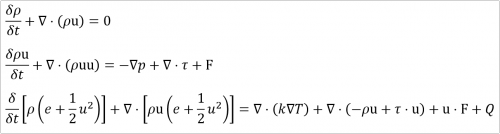

For heat transfer calculations, the temperature gradient along the dryer length indicated that heat was either carried away or added by the moving fluid (via convection) and exchanged with the dryer wall (via conduction). The temperature field was closely related to the Nusselt number, which quantifies the relationship between convective and conductive heat transfer:
- Nusselt Number
Nu = hL/k
where h is the convective heat transfer coefficient of the flow (kJ/hr-m2-K), L is the characteristic length (m), and k is the thermal conductivity of the fluid(kJ/hr-m-K).
The rotating reference frame introduces additional forces, including centrifugal and Coriolis effects, which influence the fluid flow and are accounted for using the Multiple Reference Frame (MRF) approach. This methodology is particularly effective in modeling steady-state rotating systems like the rotary dryer. Furthermore, the no-slip condition at the drum walls and the interaction with lifting flights create complex flow patterns that promote mixing and heat transfer, emphasizing the role of boundary layer theory and turbulence effects modeled through the k-ω-SST turbulence framework. These principles collectively provide a robust foundation for simulating the intricate dynamics of fluid flow and heat transfer in a rotary dryer.
The k-ω-SST turbulence model combines the advantages of the k-ε and k-ω models, providing robust predictions of turbulence in regions of free-shear flows and near-wall zones. The model uses the following transport equations:
- Turbulent Kinetic Energy (k)
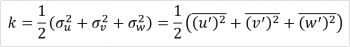
- Specific Dissipation Rate (ω)

where
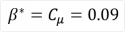
2.2. Geometry of the Rotary Dryer
The rotary dryer analyzed based on the incinerator plant at Soreang landfill consists of a cylindrical drum with a diameter of 1 m and a length of 11 m with an angle 3 degree. Internally, the drum is equipped with lifting flights designed to enhance heat and mass transfer by promoting the mixing of the fluid and particles. The inner cylinder in Figure below is designated as the rotational speed of the drum which was set to 12 rpm, consistent with industrial operation parameters. The inlet and outlet sections were designed to accommodate uniform flow distribution, with a designated fluid inlet velocity of 0.3 m/s and a temperature of 823.15 K. The drum wall was modeled as total temperature changes at the wall to simulate the thermal boundary conditions.
The rotating geometry was employed to simulate the effects of rotation without explicitly modeling transient motion using Multiple Reference Frame (MRF) method. This approach assumes a steady-state solution and divides the computational domain into rotating and stationary zones. The MRF method is computationally efficient and ideal for simulating steady-rotating machinery like the rotary dryer. The coordinate center and rotation axis of mesh rotation must be defined. The drum and lifting flights are included in the rotating zone, defined with a constant angular velocity (ω) in rad/s.

3D Geometry of rotary dryer
The actual size was scaled to 1:100 cm to enable easier and faster simulations. The computational domain was discretized using a structured mesh generated via BlockMesh/SnappyHexMesh in OpenFOAM. The geometry meshing process is assisted by the visualfoam.com meshing GUI application. Changes are made to the snappyHexMeshDict file in the system folder by modifying the refinementSurfaces function as follows.
   refinementSurfaces
   {
       Wall
       {
           level (1 1);
       }
       MRF
       {
           level (1 1);
           cellZone cellMRFzone;
           faceZone faceMRFzone;
           cellZoneInside inside;
           faceType internal;
       }
   }
Fine meshing was applied near the drum’s walls and lifting flights to capture boundary layer effects and localized gradients accurately. A mesh independence study was performed to ensure that the simulation results were not influenced by mesh size. The optimal mesh size was selected to balance accuracy and computational efficiency. Prism layers were added near solid walls to resolve near-wall turbulence effects, ensuring that the dimensionless wall distance (y+) remained within the acceptable range for the turbulence model.


Meshing results of rotary dryer
2.3. Mesh Dependence
To ensure the accuracy and reliability of the simulation results, a mesh dependence study was conducted using four different mesh configurations. The number of elements for each configuration varied significantly across hexahedral, prism, and polyhedral elements, as shown in Table 1. The study evaluated the temperature difference as the primary parameter to assess convergence.
| Hexahedrals | Prisms | Polyhedrals | Temperature Difference | |
|---|---|---|---|---|
| Meshing I | 209,348 | 15,744 | 16,764 | 8.42 % |
| Meshing II | 327,270 | 24,110 | 26,712 | 11.11 % |
| Meshing III | 1,010,382 | 61,514 | 87,719 | 2.07 % |
| Meshing IV | 1,649,544 | 106,139 | 139,514 | 0 % |

Mesh dependence study of temperature difference at 100s
2.4. Simulation Setup
In this process, the simulation setup is carried out by determining boundary conditions and some properties. The simulation utilized the buoyantSimpleFoam solver in OpenFOAM, designed for steady-state, buoyancy-driven flows involving heat transfer. The simulation code is also included so that it can be tested later. In addition, there is a video tutorial to facilitate the work steps.
2.4.1. Governing Equations
The governing equations solved by this solver are:
- Continuity Equation∇⋅(ρu) = 0
- Momentum Equation
∇⋅(ρuu) = −∇prgh+ ∇⋅τ + ρg
where prgh = p – ρgh is the pressure modified for hydrostatic balance, and g represents gravitational acceleration.
- Energy Equation
∇⋅(ρuh) = ∇⋅(α∇h) + Sh
where h is the enthalpy, α is the thermal diffusivity, and Sh represents volumetric heat sources or sinks.
The k-ω-SST turbulence model was employed to capture the turbulence effects in the flow. This model is suitable for buoyant and near-wall turbulence phenomena, ensuring accurate predictions of thermal and velocity gradients near the rotating dryer and lifting flights.
2.4.2. Boundary and Initial Conditions
- Inlet Boundary:
• Velocity: Uniform inlet velocity of 0.3 m/s.
• Temperature: Specified inlet temperature of 823.15 K.
• Turbulence Quantities: Values of turbulent kinetic energy (k) and specific dissipation rate (ω) were calculated based on flow parameters.
- Outlet Boundary:
• Pressure: Fixed pressure of 5 bar outlet condition.
• Temperature: Zero-gradient condition to allow free outflow of thermal energy.
- Wall Boundary:
• Drum Walls: No-slip condition with rotational velocity specified to match the drum’s operating speed.
• Heat Transfer: The drum wall was modeled with a zeroGradient condition, with a wall temperature changing over time.
• Lift Flights: Treated as part of the non-rotating boundary to simulate their interaction with the fluid and rotating mesh.
- Rotating Mesh:
The Multiple Reference Frame (MRF) method was employed to simulate the effects of rotation without explicitly modeling transient motion. This approach assumes a steady-state solution and divides the computational domain into rotating and stationary zones. The MRF method is computationally efficient and ideal for simulating steady rotating machinery like the rotary dryer.
• The drum and lifting flights were included in the rotating zone, defined with a constant angular velocity (ω).
• The inlet, outlet, and stationary walls were assigned to a stationary zone.
• Momentum equations within the rotating zone included Coriolis and centrifugal force terms to account for rotation effects.
• The rotational speed of the drum in radians per second (ω=2πN/60), where N = 12 RPM (the drum speed in RPM).
• The axis of rotation, typically aligned with the drum’s longitudinal axis.
• The boundaries separating the rotating and stationary zones must be defined explicitly in the mesh.
• Automatically included in the MRF formulation based on the angular velocity and rotational axis.
- Buoyancy effects:
Buoyancy effects were modeled using the Boussinesq approximation:
ρ=ρ0[1−β(T−T0)]
where β is the thermal expansion coefficient, T0 is the reference temperature, and ρ0 is the reference density.
- Numerical Schemes:
The numerical schemes were set to ensure stability and accuracy:
• Gradient Schemes: Gauss linear.
• Divergence Schemes: Gauss upwind for convection terms.
• Pressure-Velocity Coupling: SIMPLE algorithm for steady-state convergence.
• Relaxation Factors: Applied to pressure, velocity, and temperature for stable iterations.
• Convergence Criteria: Residuals for continuity, momentum, and energy were monitored, with convergence declared when residuals fell below 10−6.
* alphat
dimensions [1 -1 -1 0 0 0 0];
internalField uniform 0;
boundaryField
{
   Wall
   {
       type            compressible::alphatWallFunction;
       Prt             0.85;
       value           uniform 0;
   }
   inlet
   {
       type            calculated;
       value           $internalField;
   }
   outlet
   {
       type            calculated;
       value           $internalField;
   }
}
* k
dimensions [0 2 -2 0 0 0 0];
internalField uniform 3.75e-04;
boundaryField
{
   Wall
   {
       type            kqRWallFunction;
       value           uniform 3.75e-04;
   }
   inlet
   {
       type            fixedValue;
       value           uniform 0.001;
   }
   outlet
   {
       type            inletOutlet;
       inletValue      $internalField;
   }
}
* nut
dimensions [0 2 -1 0 0 0 0];
internalField uniform 0;
boundaryField
{
   Wall
   {
       type            nutkWallFunction;
       value           uniform 0;
   }
   inlet
   {
       type            calculated;
       value           $internalField;
   }
   outlet
   {
       type            calculated;
       value           $internalField;
   }
}
* omega
dimensions [0 0 -1 0 0 0 0];
internalField uniform 0.12;
boundaryField
{
   Wall
   {
       type            omegaWallFunction;
       value           uniform 0.12;
   }
   inlet
   {
       type            fixedValue;
       value           uniform 0.001;
   }
   outlet
   {
       type            inletOutlet;
       inletValue      $internalField;
   }
}
* p
dimensions [1 -1 -2 0 0 0 0];
internalField uniform 5e5;
boundaryField
{
   Wall
   {
       type            calculated;
       value           $internalField;
   }
   inlet
   {
       type            calculated;
       value           $internalField;
   }
   outlet
   {
       type            calculated;
       value           $internalField;
   }
}
* p_rgh
dimensions [1 -1 -2 0 0 0 0];
internalField uniform 5e5;
boundaryField
{
   Wall
   {
       type            zeroGradient;
   }
   inlet
   {
       type            zeroGradient;
   }
   outlet
   {
       type            fixedValue;
       value           uniform 5e5;
   }
}
* T
dimensions [0 0 0 1 0 0 0];
internalField uniform 293;
boundaryField
{
   Wall
   {
       type            zeroGradient;
   }
   inlet
   {
       type            fixedValue;
       value           uniform 823.15; // 550 degC
   }
   outlet
   {
       type            zeroGradient;
   }
}
* U
dimensions [0 1 -1 0 0 0 0];
internalField uniform (0 0 0);
boundaryField
{
   Wall
   {
       type            noSlip;
   }
   inlet
   {
       type            fixedValue;
       value           uniform (0.3 0 0);
   }
   outlet
   {
       type            zeroGradient;
   }
}
2.4.2. Properties
* g
dimensions [0 1 -2 0 0 0 0];
value (0 -9.81 0);
* MRFProperties
MRF
{
   cellZone    cellMRFzone;
   active      yes;
   nonRotatingPatches (Wall);
   origin    (0 0 0);
   axis      (0 0 1);
   omega     1.256637;
}
* thermophysicalProperties
thermoType {
   type            heRhoThermo;
   mixture         pureMixture;
   transport       const;
   thermo          hConst;
   equationOfState perfectGas;
   specie          specie;
   energy          sensibleEnthalpy;
}
mixture {
   specie
   {
       molWeight       28.96;
   }
   thermodynamics
   {
       Cp              1004.4;
       Hf              0;
   }
   transport
   {
       mu              1.831e-05;
       Pr              0.705;
   }
}
* turbulenceProperties
simulationType RAS;
RAS {
   RASModel            kOmegaSST;
   turbulence          on;
   printCoeffs         on;
}
3. Results and Discussion
This section presents the numerical results of the computational fluid dynamics (CFD) simulations, showcasing the time evolution of pressure (P), velocity magnitude (U Magnitude), and temperature (T) distributions inside the domain. The results are analyzed at three specific time instances: t = 50 s, t = 1000 s, and t = 2075 s, to capture transient behaviors and the approach to a quasi-steady state.
Pressure
The evolution of the pressure field is depicted in Figure 1. At t = 50 s, the pressure field exhibits distinct regions of higher and lower pressure, indicating significant gradients in the flow. The presence of oscillations at this early stage suggests the onset of an unsteady flow regime due to initial conditions or transient development. As the simulation progresses, the pressure field stabilizes. By t = 1000 s, the oscillations reduce, indicating a smoother distribution along the domain. At t = 2075 s, the pressure achieves near-uniformity with only minor spatial variations, signifying that the flow has reached a quasi-steady state.

Pressure distribution at different times
Velocity
The velocity magnitude field, visualized in Figure 2, demonstrates the development of flow uniformity over time. At t = 50 s, the velocity field is characterized by significant turbulence, with high-frequency variations visible throughout the domain. This is indicative of initial flow disturbances and strong mixing. By t = 1000 s, the fluctuations in velocity reduce substantially, and the flow transitions towards a laminar-like state. At t = 2075 s, the velocity field exhibits a nearly constant magnitude across the domain, confirming the stabilization of the flow regime.

Velocity profile at different times
Temperature
The temperature evolution, presented in Figure 3, highlights the thermal behavior within the domain. At t = 50 s, the temperature field is highly non-uniform, with localized high-temperature zones forming near specific regions. This suggests thermal gradients driven by initial flow conditions or imposed boundary conditions. As time progresses, at t = 1000 s, the temperature field begins to level out, with gradual mixing evident along the domain. By t = 2075 s, the temperature distribution stabilizes, exhibiting a clear gradient along the domain’s length, consistent with the heat transfer mechanisms governing the simulation.

Temperature distribution at different times
The results demonstrate a clear transition from an initial transient phase to a quasi-steady-state condition for all fields. The pressure distribution stabilizes first, followed by the velocity and temperature fields. This behavior aligns with expectations for such simulations, where pressure variations tend to diminish faster due to incompressibility constraints or the dominance of pressure-driven flow stabilization. The velocity and temperature results illustrate the interplay between momentum and thermal diffusion. The observed stabilization of the velocity magnitude and the gradual formation of a thermal gradient reflect the dissipation of turbulent kinetic energy and the establishment of a thermally stratified flow regime. Overall, the results validate the effectiveness of the numerical approach in capturing the dynamic evolution of the flow and thermal fields. The findings also provide insights into the flow behavior under transient and steady-state conditions, contributing to the understanding of heat and momentum transfer processes in similar systems.
Conclusion
This study demonstrated the effective use of Computational Fluid Dynamics (CFD) to evaluate the performance of a rotary dryer incinerator, utilizing the Moving Reference Frame (MRF) method within the OpenFOAM framework. By employing the buoyantSimpleFoam solver and an optimized meshing strategy, the simulation accurately captured the intricate dynamics of fluid flow, heat transfer, and turbulence within the system. The results revealed a smooth transition from transient to steady-state conditions, underscoring the reliability of the MRF method in simulating rotating machinery with computational efficiency. The findings highlighted the significance of mesh refinement in achieving precise predictions of pressure, velocity, and temperature distributions. Additionally, the application of the k-ω-SST turbulence model ensured accurate representation of near-wall and free-shear flow interactions, facilitating a deeper understanding of heat and momentum transfer mechanisms. The observed stabilization of thermal and flow fields provided insights into the thermal stratification and flow uniformity, critical for optimizing the rotary dryer’s design and operation. These results offer valuable guidance for enhancing the efficiency and sustainability of rotary dryer incinerators, contributing to improved waste management and reduced environmental impact. This work establishes a strong foundation for further research, including the integration of chemical reaction modeling and transient simulations to expand the applicability of the approach.
Reference
Acharya, P., Fogo, D., & McBride, C. (1996). Process challenges in rotary kiln-based incinerators in soil remediation projects. Environmental Progress, 15(4), 267–276. https://doi.org/https://doi.org/10.1002/ep.670150417
Jamaleddine, T. J., & Ray, M. B. (2010). Application of Computational Fluid Dynamics for Simulation of Drying Processes: A Review. Drying Technology, 28(2), 120–154. https://doi.org/10.1080/07373930903517458
Kriaa, W., Bejaoui, S., Mhiri, H., Le Palec, G., & Bournot, P. (2014). Study of dynamic structure and heat and mass transfer of a vertical ceramic tiles dryer using CFD simulations. Heat and Mass Transfer, 50(2), 235–251. https://doi.org/10.1007/s00231-013-1244-6
Leontidis, V., Baldas, L., & Colin, S. (2012). Numerical simulation of thermal transpiration in the slip flow regime with curved walls. International Conference on Nanochannels, Microchannels, and Minichannels, 44793, 205–212.
Liu, X., Arulraj, J., & Orso, A. (2024). A Framework for Inferring Properties of User-Defined Functions. Proceedings of the IEEE/ACM 46th International Conference on Software Engineering, 1–11.
Rindang, A., Panggabean, S., & Wulandari, F. (2019). CFD Analysis of Temperature Drying Chamber at Rotary Dryer With Combined Energy. Journal of Physics: Conference Series, 1155(1), 012037. https://doi.org/10.1088/1742-6596/1155/1/012037
Ryfa, A., Buczynski, R., Chabinski, M., Szlek, A., & Bialecki, R. A. (2014). Decoupled numerical simulation of a solid fuel fired retort boiler. Applied Thermal Engineering, 73(1), 794–804. https://doi.org/https://doi.org/10.1016/j.applthermaleng.2014.08.029
Saur, K., Mirmira, T., Karanasos, K., & Camacho-Rodríguez, J. (2022). Containerized execution of UDFs: an experimental evaluation. Proceedings of the VLDB Endowment, 15(11), 3158–3171.
Weller, H. G., Tabor, G., Jasak, H., & Fureby, C. (1998). A tensorial approach to computational continuum mechanics using object-oriented techniques. Computer in Physics, 12(6), 620–631. https://doi.org/10.1063/1.168744
Yang, S., Kong, Q., Zeng, D., Wu, S., Gong, F., & Xiao, R. (2022). Simulation research of a counter-flow rotary kiln hazardous waste incineration system. International Journal of Coal Science & Technology, 9(1), 60. https://doi.org/10.1007/s40789-022-00523-y