Difference between revisions of "Fadil Naufal Wahas"
Fadil.naufal (talk | contribs) |
Fadil.naufal (talk | contribs) |
||
| (82 intermediate revisions by the same user not shown) | |||
| Line 18: | Line 18: | ||
Pembimbing : Prof. Dr. Ir. Harinaldi, M.Eng. | Pembimbing : Prof. Dr. Ir. Harinaldi, M.Eng. | ||
| − | [[File:PWR.png]] | + | [[File:PWR.png|300px]] |
Pada kanal uap (''hot leg'') teras reaktor pada pembangkit listrik tenaga nuklir ''pressurized water reactor'' (PWR) terdapat fenomena ''counter-current flow limitation'' (CCFL) yang terjadi pada saat kondisi kecelakaan ''loss-of-coolant accident'' (LOCA). | Pada kanal uap (''hot leg'') teras reaktor pada pembangkit listrik tenaga nuklir ''pressurized water reactor'' (PWR) terdapat fenomena ''counter-current flow limitation'' (CCFL) yang terjadi pada saat kondisi kecelakaan ''loss-of-coolant accident'' (LOCA). | ||
| Line 34: | Line 34: | ||
| − | <youtube width=" | + | <youtube width="200" height="100">0i1AEMiyC7U </youtube> |
| − | == Computational Fluid Dynamics (CFD) == | + | == Computational Fluid Dynamics (CFD) Part 1 == |
| + | |||
| + | |||
| + | === Convergence and Grid Independence === | ||
| + | |||
| + | |||
| + | The two aspects that characterize a successful simulation result are convergence and grid independence. A converged solution have very small residuals – measures of the overall conservation of the flow properties. | ||
| + | |||
| + | The only way to eliminate errors due to coarseness of a grid is to perform a grid dependence study, which is a procedure of successive refinement of an initially coarse grid until certain key results do not change. Then the simulation is grid independent. A systematic search for convergent and grid-independent results forms an essential part of all high-quality CFD studies. | ||
| + | |||
| + | Reference: H. K. Versteeg and W. Malalasekera, ''An Introduction to Computational Fluid Dynamics: The Finite Volume Method.'' 2nd Edition. England: Pearson, 2007. | ||
| + | |||
| Line 47: | Line 58: | ||
| − | [[File:Cav2d case.png]] | + | [[File:Cav2d case.png|300px]] |
| Line 55: | Line 66: | ||
| − | [[File:Cav2d discret.png]] | + | [[File:Cav2d discret.png|300px]] |
| Line 61: | Line 72: | ||
| − | [[File:Cav2d u.png]] | + | [[File:Cav2d u.png|300px]] |
| − | [[File:Cav2d p.png]] | + | [[File:Cav2d p.png|300px]] |
It can be shown that the air is indeed moving inside the cavity and the air that is closest to the upper wall is also moving with the greatest magnitude. From the pressure contour, it can be seen that the upper-most-right corner has the greatest pressure. This is due to the fact that air is colliding at that corner and is diverted to the adjacent bottom. This collision occurs at the 4 corners of the wall, thus creating the swirling effect with the smallest velocity magnitude at the center of the swirl. | It can be shown that the air is indeed moving inside the cavity and the air that is closest to the upper wall is also moving with the greatest magnitude. From the pressure contour, it can be seen that the upper-most-right corner has the greatest pressure. This is due to the fact that air is colliding at that corner and is diverted to the adjacent bottom. This collision occurs at the 4 corners of the wall, thus creating the swirling effect with the smallest velocity magnitude at the center of the swirl. | ||
| + | |||
| + | |||
| + | |||
| + | === OpenFOAM Solvers === | ||
| + | |||
| + | |||
| + | Here are solvers that OpenFOAM offers. The table below classifies the solver based on the flow of the fluid and depends on the case-by-case problem. | ||
| + | |||
| + | {| class="wikitable" style="margin:auto" | ||
| + | |+ OpenFOAM Solvers | ||
| + | |- | ||
| + | ! No. !! Solver !! Algorithm !! Time !! Flow !! Compressibility !! Phase | ||
| + | |- | ||
| + | | 1 || simpleFoam || SIMPLE || Steady-State || Laminar/Turbulent || Incompressible || Single-phase | ||
| + | |- | ||
| + | | 2 || icoFoam || PISO || Transient || Laminar || Incompressible || Single-phase | ||
| + | |- | ||
| + | | 3 || pisoFoam || PISO || Transient || Turbulent || Incompressible || Single-phase | ||
| + | |- | ||
| + | | 4 || pimpleFoam || PISO+SIMPLE || Transient || Turbulent || Incompressible || Single-phase | ||
| + | |- | ||
| + | | 5 || interFoam || PISO+SIMPLE || Transient || Turbulent || Incompressible || '''Multi-phase''' | ||
| + | |- | ||
| + | | 6 || - || - || - || - || - || - | ||
| + | |} | ||
| + | |||
| + | |||
| + | SIMPLE = Semi-Implicit Method for Pressure Linked Equations | ||
| + | |||
| + | PISO = Pressure Implicit with Splitting of Operators | ||
| + | |||
| + | |||
| + | |||
| + | === Cavity 2D with OpenFOAM === | ||
| + | |||
| + | |||
| + | The problem we are trying to solve is lid-driven cavity. Same as previous case, the geometry is a 2 dimensional 0.1 m by 0.1 m (gamma = Lx/Ly = 1) cavity space with the upper wall moving to the positive x-axis direction at certain velocities. The boundary of right, left, and lower wall is stationary. The fluid is air with kinematic viscosity (nu) of 1 * 10-⁵ m²/s. | ||
| + | |||
| + | The INTENTION of this preliminary study is to understand the effect of Reynolds number (Re) on the air flow inside the lid-driven cavity, particularly the flow profile. At certain velocity, is it laminar, transitional, or turbulent? At what Reynolds number does the change occurs? | ||
| + | |||
| + | |||
| + | <math> Re = \frac{&rho U L}{&mu} = \frac{U L}{\&nu} . . . (1) </math> | ||
| + | |||
| + | |||
| + | where: | ||
| + | Re = Reynolds number (-) | ||
| + | rho = fluid density (kg/m³) | ||
| + | U = inlet velocity = upper wall velocity (m/s) | ||
| + | L = characteristic length = wall length = 0.1 m | ||
| + | mu = dynamic viscosity (kg/m-s) | ||
| + | nu = kinematic viscosity = 1 * 10-⁵ (m²/s) | ||
| + | |||
| + | Reynolds number can be calculated using the Eq. (1). We can vary the Reynolds number by varying the wall velocity. Here, the upper wall velocity is varied from 0.0001 m/s to 0.8 m/s with various increment. The wall velocity variation is presented at the table below. | ||
| + | |||
| + | |||
| + | {| class="wikitable" style="margin:auto" | ||
| + | |+ Table 1. Variation of wall velocity | ||
| + | |- | ||
| + | ! U (m/s) !! Re (-) | ||
| + | |- | ||
| + | | 0.0001 || 1 | ||
| + | |- | ||
| + | | 0.01 || 100 | ||
| + | |- | ||
| + | | 0.02 || 200 | ||
| + | |- | ||
| + | | 0.03 || 300 | ||
| + | |- | ||
| + | | 0.04 || 400 | ||
| + | |- | ||
| + | | 0.05 || 500 | ||
| + | |- | ||
| + | | 0.1 || 1000 | ||
| + | |- | ||
| + | | 0.2 || 2000 | ||
| + | |- | ||
| + | | 0.3 || 3000 | ||
| + | |- | ||
| + | | 0.8 || 8000 | ||
| + | |} | ||
| + | |||
| + | |||
| + | We used the open-source CFD software OpenFOAM for this study with simpleFoam solver for both laminar and turbulent flow, with the latter using the k-Omega turbulence model. The flow was assumed to be steady-state. A 50 by 50 hexahedral grid mesh was used in the model, where the z-axis was set to 1 cell to represent the 2 dimensional case. | ||
| + | |||
| + | First, we validated our simulation by comparing the case with U = 0.0001 m/s and U = 0.8 m/s, hence the Re are 1 and 8000, respectively, with the case from a study conducted by Hendriketal [1], also with the same Re. The fluid flow with the isolines (streamlines) from both simulation and reference [1] can be seen in the Fig. 1 and Fig. 2 below. It can be seen that the results generated by our simulations is the same as the results obtained from [1]. | ||
| + | |||
| + | |||
| + | [[File:Sim 1vs8k.png|1000px]] | ||
| + | |||
| + | |||
| + | [[File:Ref 1vs8k.png|900px]] | ||
| + | |||
| + | |||
| + | The flow with Re = 1 is laminar and almost vertically symmetrical and the flow with Re = 8000 is turbulent with 3 secondary eddies in the 3 corners of the cavity. | ||
| + | |||
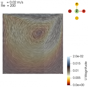
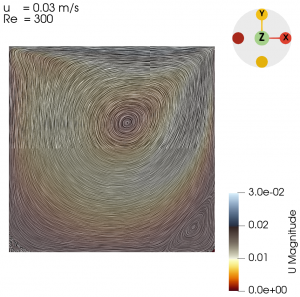
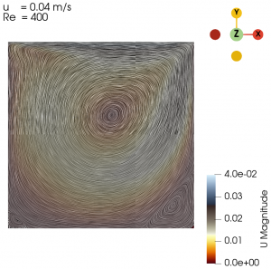
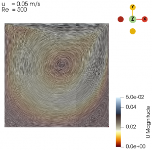
| + | Next we varied the parameter of U from 0.01 m/s to 0.3 m/s with simpleFoam laminar model as per Table 1, and look at the flow profile of the cavity. The isolines can be seen at Fig. 3 to Fig. 10. | ||
| + | |||
| + | |||
| + | [[File:1 cavity 0.01.png|300px]] [[File:2 cavity 0.02.png|300px]] [[File:3 cavity 0.03.png|300px]] [[File:4 cavity 0.04.png|300px]] [[File:5 cavity 0.05.png|300px]] [[File:6 cavity 0.1.png|300px]] [[File:7 cavity 0.2.png|300px]] [[File:8 cavity 0.3.png|300px]] | ||
| + | |||
| + | |||
| + | Convergence can be seen from simulation's variables residuals below. | ||
| + | |||
| + | Re = 1 | ||
| + | |||
| + | [[File:Residuals Initial.png|500px]] | ||
| + | |||
| + | |||
| + | Re = 8000 | ||
| + | |||
| + | [[File:Residuals Initial 0.8.png|500px]] | ||
| + | |||
| + | |||
| + | |||
| + | References: | ||
| + | |||
| + | [1] H. C. Kuhlmann and F. Romanò, "The Lid-Driven Cavity," ''Computational Methods in Applied Sciences'', vol. 50, 2019. https://doi.org/10.1007/978-3-319-91494-7_8 | ||
| + | |||
| + | |||
| + | |||
| + | === Lid-Driven Cavity with DAI5 Framework === | ||
| + | |||
| + | |||
| + | This is a video essay of the application of DAI5 Framework in understanding lid-driven cavity. The lid-driven cavity simulation is done using OpenFOAM. | ||
| + | |||
| + | Disclaimer: the video is in Bahasa Indonesia. | ||
| + | |||
| + | |||
| + | Lid-Driven Cavity Case File: [https://drive.google.com/file/d/1zm4B-IdIKUf1YTrn_xshXi5hma2PyicI/view?usp=drive_link bit.ly/CavityDAI5] | ||
| + | |||
| + | |||
| + | <youtube width="200" height="100">cn7qFkYGFXU </youtube> | ||
| + | |||
| + | |||
| + | |||
| + | == Paper Draft == | ||
| + | |||
| + | Grid Independency Study on the Turbulence of Lid Driven Cavity using DAI5 Framework | ||
| + | |||
| + | [https://drive.google.com/file/d/1XOcIdnCVsgjJ-2x3sb2RG9TVxO1NoGMC/view?usp=sharing Google Drive] | ||
| + | |||
| + | |||
| + | |||
| + | == Mid Test with ChatGPT == | ||
| + | |||
| + | |||
| + | {| class="wikitable" style="width: 99%;" | ||
| + | | style="text-align: center;" colspan="3" | '''Mid Test with ChatGPT''' | ||
| + | |- | ||
| + | | style="width: 20%;"| | ||
| + | | style="width: 80%;text-align:right; color:#ffffff; background-color:#232323; padding: 20px;" colspan="2"| '''User''' | ||
| + | |- | ||
| + | | style="width: 80%;text-align:left; color:#ffffff; background-color:#232323; padding: 20px;" colspan="2"| ChatGPT | ||
| + | | style="width: 20%;"| | ||
| + | |- | ||
| + | | style="width: 20%;"| | ||
| + | | style="width: 80%;text-align:right; color:#ffffff; background-color:#232323; padding: 20px;" colspan="2"| '''I am going to take an exam on the subject of basic Computational Fluid Dynamics (CFD). I need you to create a basic test consisted of 5 short-answer questions all at once and grade what I do.''' | ||
| + | |- | ||
| + | | style="width: 80%;text-align:left; color:#ffffff; background-color:#232323; padding: 20px;" colspan="2"| Here’s a basic test on Computational Fluid Dynamics (CFD) consisting of 5 short-answer questions: | ||
| + | |||
| + | |||
| + | CFD Basic Test | ||
| + | |||
| + | Question 1: Define the term "viscosity" and explain its significance in fluid flow. | ||
| + | |||
| + | Question 2: What is the difference between laminar and turbulent flow? Provide examples of each. | ||
| + | |||
| + | Question 3: Explain the concept of grid independence in CFD and why it is important for accurate simulation results. | ||
| + | |||
| + | Question 4: Describe the role of the Navier-Stokes equations in CFD. What do they represent? | ||
| + | |||
| + | Question 5: What are boundary conditions in CFD, and why are they crucial for setting up a simulation? | ||
| + | |||
| + | |||
| + | Once you answer these questions, I can grade your responses! | ||
| + | | style="width: 20%;"| | ||
| + | |- | ||
| + | | style="width: 20%;"| | ||
| + | | style="width: 80%;text-align:left; color:#ffffff; background-color:#232323; padding: 20px;" colspan="2"| '''1. Define the term "viscosity" and explain its significance in fluid flow.''' | ||
| + | |||
| + | Viscosity is a measure of a fluid’s internal friction or resistance to deformation or flow when a force is applied to it. It is a fluid-specific property where fluids with higher viscosity, like syrup, deform less easily compared to fluids with lower viscosity, like water. There are two types of viscosity, the dynamic viscosity (mu) and the kinematic viscosity (nu), with units kg/m.s and m^2/s, respectively. In fluid flow applications, viscosity plays a vital role in determining whether the flow is laminar or turbulent. Viscosity is a critical property that affects fluid dynamics, influencing how fluids flow and behave under various conditions. | ||
| + | |||
| + | '''2. What is the difference between laminar and turbulent flow? Provide examples of each.''' | ||
| + | |||
| + | Laminar flow is characterized by smooth, orderly motion of fluid layers, with each layer sliding past the adjacent ones with minimal to no mixing. This type of flow typically occurs at low Reynolds numbers (Re < 2000). An example of laminar flow is the flow of blood inside our capillaries or the flow of air inside a wind tunnel before contact. | ||
| + | |||
| + | Turbulent flow, on the other hand, is characterized by irregular fluid motion with significant mixing and fluctuations in velocity. This type of flow typically occurs at high Reynolds numbers (Re > 4000). An example of turbulent flow is the air in and out of our respiratory system or the airflow around an airplane wing. | ||
| + | |||
| + | '''3. Explain the concept of grid independence in CFD and why it is important for accurate simulation results.''' | ||
| + | |||
| + | Grid independence refers to the condition where the results of a simulation do not significantly change with further refinement of the computational grid (mesh). This can be done with a grid dependence study, which is a procedure of successive refinement of an initially coarse grid until certain key results do not change. Achieving grid independence is crucial because it ensures that the numerical solution is not influenced by the discretization of the domain, leading to more reliable and accurate results. A systematic search for grid-independent result forms an essential part of all high-quality CFD studies. | ||
| + | |||
| + | '''4. Describe the role of the Navier-Stokes equations in CFD. What do they represent?''' | ||
| + | |||
| + | The Navier-Stokes equations are a set of nonlinear partial differential equations that describe the motion of fluid. They represent the conservation of momentum in fluid flow and are fundamental to the field of computational fluid dynamics. The equations account for viscosity, pressure, and external forces acting on the fluid. In CFD, solving the Navier-Stokes equations enables the prediction of velocity fields, pressure distributions, and other flow characteristics, making them essential for simulating and analyzing fluid behavior in various engineering applications. | ||
| + | |||
| + | '''5. What are boundary conditions in CFD, and why are they crucial for setting up a simulation?''' | ||
| + | |||
| + | Boundary conditions in CFD define the behavior of the fluid at the boundaries of the computational domain. They specify values for variables such as velocity, pressure, and other relevant quantities at the edges of the simulation space. They ensure that the simulation reflects the physical reality of the problem being modeled, allowing for accurate predictions and are essential for producing valid and reliable CFD results. | ||
| + | |- | ||
| + | | style="width: 80%;text-align:left; color:#ffffff; background-color:#232323; padding: 20px;" colspan="2"| Grading: | ||
| + | |||
| + | * Definition of Viscosity: (9/10) | ||
| + | |||
| + | Your explanation is clear and well-structured. You correctly define viscosity and its types (dynamic and kinematic) along with their units. You also mention its importance in fluid dynamics and how it affects flow behavior. | ||
| + | One minor note: You could expand on how viscosity affects energy dissipation in the flow. Nonetheless, your answer is quite strong. | ||
| + | |||
| + | * Difference between Laminar and Turbulent Flow: (10/10) | ||
| + | |||
| + | Excellent explanation of both laminar and turbulent flows with clear examples and correct references to Reynolds numbers. The distinction between orderly and chaotic motion is well articulated, and the examples are accurate. | ||
| + | |||
| + | * Grid Independence Concept: (10/10) | ||
| + | |||
| + | Great explanation! You correctly identify grid independence and explain the grid dependence study and its importance in ensuring simulation accuracy. This is a key concept in CFD, and your description captures it thoroughly. | ||
| + | |||
| + | * Role of Navier-Stokes Equations: (10/10) | ||
| + | |||
| + | Your answer effectively highlights the significance of the Navier-Stokes equations in CFD. You mention their role in momentum conservation, accounting for viscosity, pressure, and forces, and how they are used to predict key flow characteristics. This is a complete and concise answer. | ||
| + | |||
| + | * Boundary Conditions in CFD: (9/10) | ||
| + | |||
| + | Good explanation of boundary conditions and their role in simulations. You correctly mention their importance in defining variables at the boundaries and ensuring physical realism in the model. | ||
| + | A small suggestion: you could briefly touch upon specific types of boundary conditions (e.g., Dirichlet, Neumann) for more depth, but your answer is still very solid. | ||
| + | |||
| + | '''Overall Score: 96/100''' | ||
| + | |||
| + | Excellent work! Your understanding of CFD fundamentals is strong, and you provided clear, well-articulated answers throughout the test. Just minor improvements in elaboration could make it even better. | ||
| + | | style="width: 20%;"| | ||
| + | |- | ||
| + | | style="width: 20%;"| | ||
| + | | style="width: 80%;text-align:right; color:#ffffff; background-color:#232323; padding: 20px;" colspan="2"| '''How does viscosity affects energy dissipation in the fluid flow? Could you elaborate?''' | ||
| + | |- | ||
| + | | style="width: 80%;text-align:left; color:#ffffff; background-color:#232323; padding: 20px;" colspan="2"| Viscosity affects energy dissipation in fluid flow by resisting the motion of fluid layers, converting kinetic energy into thermal energy (heat) through internal friction. Here’s how this process works in detail: | ||
| + | |||
| + | Internal Friction and Shear Stress: Viscosity causes internal friction between adjacent layers of fluid moving at different velocities. This friction leads to shear stress, which requires energy to maintain. As layers slide past each other, some of the flow’s kinetic energy is “used up” in overcoming this frictional resistance. | ||
| + | |||
| + | Conversion of Kinetic Energy to Heat: The energy needed to overcome the viscous forces does not just vanish; it’s transformed into heat. This phenomenon is known as viscous dissipation. In regions with high velocity gradients (such as near solid boundaries in turbulent flows), the energy dissipation rate is higher, causing more kinetic energy to be converted to heat. | ||
| + | |||
| + | Impact on Flow Types: | ||
| + | |||
| + | Laminar Flow: In low-viscosity, laminar flows, this energy dissipation is relatively low, as the layers slide smoothly over each other. However, viscosity is still crucial for determining the flow regime and ensuring the orderly motion of fluid layers. | ||
| + | Turbulent Flow: In turbulent flows, viscosity plays a larger role in dissipating energy. The chaotic, fluctuating motion of fluid particles in turbulence generates numerous small eddies, which further increase the velocity gradients and amplify the energy dissipation through viscous effects. | ||
| + | Implications in Engineering and CFD: High-viscosity fluids dissipate more energy as heat, which can be critical for cooling and lubrication applications. In CFD, accurately modeling viscosity is essential to capture realistic energy dissipation, especially in simulations involving turbulent flows, as it affects flow stability, boundary layer characteristics, and even heat transfer predictions. | ||
| + | |||
| + | Understanding viscosity's role in energy dissipation is crucial for designing efficient fluid systems, as well as for accurately predicting fluid behavior in simulations. | ||
| + | | style="width: 20%;"| | ||
| + | |- | ||
| + | | style="width: 20%;"| | ||
| + | | style="width: 80%;text-align:right; color:#ffffff; background-color:#232323; padding: 20px;" colspan="2"| '''What are the Dirichlet and Neumann boundary conditions? What other types of boundary conditions are there?''' | ||
| + | |- | ||
| + | | style="width: 80%;text-align:left; color:#ffffff; background-color:#232323; padding: 20px;" colspan="2"| In CFD, boundary conditions define how fluid behaves at the edges of the simulation domain. Here’s a breakdown of Dirichlet and Neumann boundary conditions, along with a few other common types: | ||
| + | |||
| + | * Dirichlet Boundary Condition (Fixed Value): | ||
| + | |||
| + | This boundary condition specifies a fixed value for a field variable (like velocity, pressure, or temperature) at the boundary. | ||
| + | For instance, setting the temperature on a wall to a constant value (e.g., 300 K) or prescribing a fixed velocity at an inlet. | ||
| + | Dirichlet conditions are commonly used to impose known values at inflow boundaries or solid surfaces with a constant temperature. | ||
| + | |||
| + | * Neumann Boundary Condition (Fixed Gradient or Flux): | ||
| + | |||
| + | This condition specifies a fixed rate of change, or gradient, of a variable at the boundary rather than the variable's value itself. | ||
| + | For example, setting the heat flux across a wall surface to a constant (which relates to the temperature gradient) or defining a zero-velocity gradient (indicating no shear stress). | ||
| + | Neumann conditions are often applied when the exact value is unknown, but the flux or rate of change at the boundary is known, such as insulated walls (zero heat flux) or stress-free outflows. | ||
| + | |||
| + | * Robin (Mixed) Boundary Condition: | ||
| + | |||
| + | This combines aspects of Dirichlet and Neumann conditions by defining a relationship between the variable and its gradient at the boundary. | ||
| + | For instance, in heat transfer, it can represent convective cooling, where the heat flux is proportional to the temperature difference between the fluid and the boundary (e.g., Newton's Law of Cooling). | ||
| + | Robin conditions are used in situations where the boundary value depends on both the internal variable and its rate of change, such as semi-permeable membranes or convective heat transfer. | ||
| + | |||
| + | * Periodic Boundary Condition: | ||
| + | |||
| + | This boundary condition enforces a repeating pattern in space, where the variables on one side of the boundary match those on the opposite side. | ||
| + | For example, in simulations of flow over a regularly spaced array of objects, where the pattern of flow repeats, periodic conditions allow efficient modeling by simulating just a small section. | ||
| + | This is especially useful in simulations of channels, waves, and symmetric or repeating systems. | ||
| + | |||
| + | * Symmetry Boundary Condition: | ||
| + | |||
| + | This condition is applied when the domain has a plane of symmetry, where no flow or gradient exists normal to the symmetry plane. | ||
| + | The symmetry boundary implies that the normal component of velocity and the normal gradient of scalar variables (like pressure or temperature) are zero. | ||
| + | Useful for reducing computational load by only simulating half or a section of a symmetric geometry, like a cylindrical pipe. | ||
| + | |||
| + | * Outflow (or Far-Field) Boundary Condition: | ||
| + | |||
| + | Designed for flow exiting the domain, where minimal influence from the boundary on the internal flow is desired. Outflow boundaries often enforce zero gradients or “do-nothing” conditions to allow fluid to exit freely. | ||
| + | In external flow problems, like around an airplane, far-field conditions simulate an open, infinite environment where variables gradually return to ambient values as they move away from the body. | ||
| + | |||
| + | Each type of boundary condition serves a specific purpose, helping to set up simulations that accurately reflect real physical scenarios. The choice of boundary condition is crucial as it significantly affects simulation stability and results accuracy. | ||
| + | | style="width: 20%;"| | ||
| + | |} | ||
| + | |||
| + | |||
| + | '''Self-Assessment''' | ||
| + | |||
| + | I feel like I learned a lot in this CFD Application class. To me, the Navier-Stokes and its numerical solution are substantial in CFD. I can understand more about the concept and theory of CFD and apply them in an analysis. Based on this self-assessment of my performance, I believe I have met the expectations and objectives of the class thus far, which I feel merits a self-assessment score of 92 out of 100. | ||
| + | |||
| + | |||
| + | '''Post-Mid Test Plan for the Class''' | ||
| + | |||
| + | It would be nice to know more about the heat transfer aspects of computational fluid dynamics and how to apply it in a case problem. | ||
| + | |||
| + | |||
| + | |||
| + | == Computational Fluid Dynamics (CFD) Part 2 == | ||
| + | |||
| + | |||
| + | === Temperature-Difference-Driven Cavity === | ||
| + | |||
| + | |||
| + | We try to replicate the study conducted by Betts and Bokhari. Here, we have a rectangular cavity with the dimensions of 0.076 m x 0.52 m x 2.18 m in the x, y, and z axis, respectively, as seen in the figure below. There are no lids in this cavity. Rather, the cavity is driven by temperature difference. The right wall is constantly heated to 39.9 °C, while the left wall is constantly heated to 19.6 °C. | ||
| + | |||
| + | |||
| + | [[File:CavHT geo.png|200px]] | ||
| + | |||
| + | |||
| + | The objective of this study is to understand the fluid flow (in this case, air) due to the temperature difference. The assumptions are the flow is in steady-state. The study is done using OpenFOAM with buoyantSimpleFoam solver with kOmegaSST turbulence model. Rather than specifying the velocity in the boundary condition, the case will have temperature in the boundary condition. The case file can be downloaded from [https://develop.openfoam.com/Development/openfoam/-/tree/master/tutorials/heatTransfer/buoyantSimpleFoam/buoyantCavity buoyantCavity] | ||
| + | |||
| + | |||
| + | [[File:CavHT T.png|200px]] [[File:CavHT full.png|200px]] | ||
| + | |||
| + | |||
| + | It can be seen from the 2 images above that there exist a temperature difference on the right and left walls. This temperature difference lead to the flow of the air inside the cavity. The flow of the air inside the cavity resembles the elongated vortex that can be seen more detailed in the zoomed-in images below. | ||
| + | |||
| + | |||
| + | [[File:CavHT vec top.png|400px]] [[File:CavHT vec bottom.png|400px]] | ||
| + | |||
| + | |||
| + | If we look at the velocity profile in the y axis direction in the centerline of the cavity, we can be certain that there exist a vortex inside the cavity. The velocity profile can be seen in the images below, with a close comparison to the study conducted by Betts and Bokhari. | ||
| + | |||
| + | [[File:CavHT vy cfd.png|400px]] [[File:CavHT vy exp.png|200px]] | ||
| + | |||
| + | |||
| + | Reference: P.L. Betts, I.H. Bokhari, "Experiments on turbulent natural convection in an enclosed tall cavity," ''International Journal of Heat and Fluid Flow'', vol. 21, pp. 675-683, 2000. | ||
| + | |||
| + | |||
| + | |||
| + | === Lid-Driven Cavity with Artificial Neural Network (ANN) === | ||
| + | |||
| + | |||
| + | Using the data from the previous study [https://air.eng.ui.ac.id/index.php?title=Fadil_Naufal_Wahas#Cavity_2D_with_OpenFOAM Cavity 2D with OpenFOAM], we gather 4 variations of lid velocity of the cavity, 0.01, 0.05, 0.1, 0.3 m/s. With this 4 variations of velocity, along with the x and y coordinates of the cells of the control volume of the 50x50 grid cavity (the mesh cells), we can gather the 10,000 rows of data as the input for the ANN modeling with the pressure (p), x-axis velocity component (Ux), and y-axis velocity component (Uy) in said coordinate as the output of the ANN modeling. | ||
| + | |||
| + | The simulation files, the input-output table, and the Python codes can be downloaded [https://drive.google.com/file/d/17O5dGe-nzPish4UBVywYLVmXl7F4PVSH/view?usp=sharing here]. | ||
| + | |||
| + | From the ANN modeling with 2 hidden layers and 128 neurons per hidden layer, as seen in the ANN Architecture below, and 500 epochs, it can be seen that the evaluation of the model yields relatively good results. | ||
| + | |||
| + | |||
| + | [[File:1 ANN Architecture.png|400px]] | ||
| + | |||
| + | |||
| + | The ANN modeling resulted in the model loss of less than 5e-4 as seen below. | ||
| + | |||
| + | |||
| + | [[File:2 Model Loss.png|300px]] | ||
| + | |||
| + | |||
| + | The ANN model can predict the p, Ux, and Uy with coefficient of determination (R²) of more than 0.985, 0.975, and 0.99, respectively, as seen below. | ||
| + | |||
| + | |||
| + | [[File:Act vs Pred 1.png|300px]] [[File:Act vs Pred 2.png|300px]] [[File:Act vs Pred 3.png|300px]] | ||
| + | |||
| + | |||
| + | This is further supported by the visualization of the airflow inside the cavity. Here, we compare the velocity vector field of lid-driven cavity with the lid moving at 0.1 m/s, both the simulation (actual data) and the ANN prediction (predicted data) | ||
| + | |||
| + | |||
| + | [[File:Vector field 0.1.png|350px]] [[File:6 cavity 0.1.png|300px]] | ||
| + | |||
| + | |||
| + | This result can of course be improved by varying the ANN modeling parameters such as the number of hidden layer, the number of neurons per hidden layer, and the number of epoch, and also adding more and more data from the variations of simulation to cover a broader range of conditions. | ||
| + | |||
| + | |||
| + | |||
| + | === Discussion with ChatGPT: Continuum Mechanics === | ||
| + | |||
| + | |||
| + | {| class="wikitable" style="width: 99%;" | ||
| + | | style="text-align: center;" colspan="3" | '''Continuum Mechanics''' | ||
| + | |- | ||
| + | |- | ||
| + | | style="width: 20%;"| | ||
| + | | style="width: 80%;text-align:left; color:#ffffff; background-color:#232323; padding: 10px;" colspan="2"| USER | ||
| + | |- | ||
| + | | style="width: 80%;text-align:left; color:#ffffff; background-color:#232323; padding: 10px;" colspan="2"| AI | ||
| + | | style="width: 20%;"| | ||
| + | |- | ||
| + | | style="width: 20%;"| | ||
| + | | style="width: 80%;text-align:left; color:#ffffff; background-color:#232323; padding: 20px;" colspan="2"| Can you give a practical example (along with a simple calculator for a 1D problem) in engineering where continuum mechanics treats materials as continuous, focusing on the integration of an uninterrupted 'conscious continuum' into the DAI5 framework. | ||
| + | |- | ||
| + | | style="width: 80%;text-align:left; color:#ffffff; background-color:#232323; padding: 20px;" colspan="2"| Certainly! Continuum mechanics simplifies the study of materials by assuming they are continuous and devoid of voids, even though materials are composed of discrete particles. This assumption allows engineers to use mathematical tools, such as differential equations and integration, to analyze stresses, strains, and material behavior. Let’s create a practical example in engineering: | ||
| + | |||
| + | Problem: 1D Axial Deformation of a Rod | ||
| + | A steel rod of length L=1.0m, cross-sectional area A=0.01m², and Young's modulus E=200GPa is subjected to a tensile force F=10,000N. The goal is to calculate the elongation ΔL of the rod using continuum mechanics and integrate it with the DAI5 framework as an uninterrupted "conscious continuum." | ||
| + | |||
| + | Continuum Mechanics Solution: | ||
| + | Using the 1D axial deformation formula: | ||
| + | |||
| + | ΔL=FL/AE | ||
| + | |||
| + | where F = Applied force, L = Original length, A = Cross-sectional area, E = Young's modulus | ||
| + | |||
| + | DAI5 Framework Integration: | ||
| + | |||
| + | Intention: Understand how a tensile force deforms a continuous rod in 1D. | ||
| + | |||
| + | Initial Thinking: Assume a linear elastic behavior where stress and strain follow Hooke's Law. Define the rod as a continuum, ignoring atomic-scale irregularities. | ||
| + | |||
| + | Idealization: Use the governing equation derived from Hooke’s Law, treating material properties as constant and uniformly distributed. | ||
| + | |||
| + | Instruction Set: Write a program to calculate the elongation and visualize its dependence on F, A, E, and L. | ||
| + | |||
| + | |||
| + | Python Calculator: | ||
| + | |||
| + | F = 10000 # Force in Newtons | ||
| + | |||
| + | L = 1.0 # Length in meters | ||
| + | |||
| + | A = 0.01 # Cross-sectional area in square meters | ||
| + | |||
| + | E = 200e9 # Young's modulus in Pascals | ||
| + | |||
| + | delta_L = (F * L) / (A * E) | ||
| + | |||
| + | print(f"Elongation (ΔL): {delta_L:.6f} m") | ||
| + | |||
| + | | style="width: 20%;"| | ||
| + | |} | ||
| + | |||
| + | |||
| + | |||
| + | === Reduced-Order Model (ROM) using Python: 1D Conduction === | ||
| + | |||
| + | |||
| + | ''In Progress.'' | ||
| + | |||
| + | |||
| + | |||
| + | === Reduced-Order Model (ROM) using ITHACA-FV: Backward Facing Step (PitzDaily) === | ||
| + | |||
| + | |||
| + | ''In Progress.'' | ||
| + | |||
| + | |||
| + | |||
| + | (EOF) | ||
Latest revision as of 21:29, 19 November 2024
Assalamu'alaikum Warahmatullahi Wabarakatuh, Salam Sejahtera untuk kita semua.
Perkenalkan, saya Fadil Naufal Wahas, NPM 2306185416, mahasiswa magister Departemen Teknik Mesin Universitas Indonesia.
Contents
Thesis
Tesis : Studi komputasi tentang pengaruh sifat fluida terhadap karakteristik counter-current flow limitation (CCFL) di 1/30 pressurized water reactor (PWR) hot leg
Thesis : Computational study of the effects of fluid properties on counter-current flow limitation (CCFL) characteristics in 1/30 pressurized water reactor (PWR) hot leg
Pembimbing : Prof. Dr. Ir. Harinaldi, M.Eng.
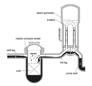
Pada kanal uap (hot leg) teras reaktor pada pembangkit listrik tenaga nuklir pressurized water reactor (PWR) terdapat fenomena counter-current flow limitation (CCFL) yang terjadi pada saat kondisi kecelakaan loss-of-coolant accident (LOCA).
Saat LOCA, karena adanya penurunan tekanan, terjadi penguapan air pendingin yang berada di reaktor sehingga uap tersebut mengalir ke steam generator (SG) melalui hot leg. Sebagian uap yang terkumpul di SG tersebut mengalami kondensasi menjadi air. Air tersebut, dipengaruhi gravitasi, mengalir kembali ke reaktor, berlawanan arah dengan uap. Aliran berlawanan arah ini terjadi saat kecepatan aliran uap berada di bawah ambang batas flooding atau counter-current flow limitation (CCFL).
Fenomena CCFL ini menjadi penting untuk diteliti karena berhubungan dengan keselamatan reaktor nuklir. Oleh karena itu, pengaruh sifat fisik fluida terhadap karakteristik CCFL perlu diinvestigasi.
DAI5 Framework
DAI5 Framework is a guideline developed by Dr. Ahmad Indra Siswantara for problem-solving processes. This video essay is my interpretation of the DAI5 Framework.
Computational Fluid Dynamics (CFD) Part 1
Convergence and Grid Independence
The two aspects that characterize a successful simulation result are convergence and grid independence. A converged solution have very small residuals – measures of the overall conservation of the flow properties.
The only way to eliminate errors due to coarseness of a grid is to perform a grid dependence study, which is a procedure of successive refinement of an initially coarse grid until certain key results do not change. Then the simulation is grid independent. A systematic search for convergent and grid-independent results forms an essential part of all high-quality CFD studies.
Reference: H. K. Versteeg and W. Malalasekera, An Introduction to Computational Fluid Dynamics: The Finite Volume Method. 2nd Edition. England: Pearson, 2007.
Cavity 2D Laminar Flow with CFDSOF
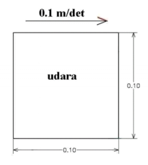
The image below shows a 0.1 m by 0.1 m cavity section filled with air (udara) where the upper wall is moving in the +x-axis direction at 0.1 m/s where the density (ρ) of air is 1 kg/m^3, the dynamic viscosity (µ) of air is 2 * 10^-5 kg/m-s, and the flow is laminar, i.e. Re = 500.
The grid-structured *CFDSOF* software is used in this simulation case.
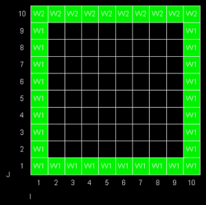
First, cavity is discritized by dividing it into cells, in this case, a 10x10 cells.
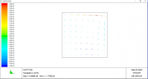
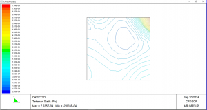
Then, after specifying the boundary condition of the walls and the iteration of the case, the iteration begins. The results of the velocity vector field and the pressure contour are shown in the images below.
It can be shown that the air is indeed moving inside the cavity and the air that is closest to the upper wall is also moving with the greatest magnitude. From the pressure contour, it can be seen that the upper-most-right corner has the greatest pressure. This is due to the fact that air is colliding at that corner and is diverted to the adjacent bottom. This collision occurs at the 4 corners of the wall, thus creating the swirling effect with the smallest velocity magnitude at the center of the swirl.
OpenFOAM Solvers
Here are solvers that OpenFOAM offers. The table below classifies the solver based on the flow of the fluid and depends on the case-by-case problem.
| No. | Solver | Algorithm | Time | Flow | Compressibility | Phase |
|---|---|---|---|---|---|---|
| 1 | simpleFoam | SIMPLE | Steady-State | Laminar/Turbulent | Incompressible | Single-phase |
| 2 | icoFoam | PISO | Transient | Laminar | Incompressible | Single-phase |
| 3 | pisoFoam | PISO | Transient | Turbulent | Incompressible | Single-phase |
| 4 | pimpleFoam | PISO+SIMPLE | Transient | Turbulent | Incompressible | Single-phase |
| 5 | interFoam | PISO+SIMPLE | Transient | Turbulent | Incompressible | Multi-phase |
| 6 | - | - | - | - | - | - |
SIMPLE = Semi-Implicit Method for Pressure Linked Equations
PISO = Pressure Implicit with Splitting of Operators
Cavity 2D with OpenFOAM
The problem we are trying to solve is lid-driven cavity. Same as previous case, the geometry is a 2 dimensional 0.1 m by 0.1 m (gamma = Lx/Ly = 1) cavity space with the upper wall moving to the positive x-axis direction at certain velocities. The boundary of right, left, and lower wall is stationary. The fluid is air with kinematic viscosity (nu) of 1 * 10-⁵ m²/s.
The INTENTION of this preliminary study is to understand the effect of Reynolds number (Re) on the air flow inside the lid-driven cavity, particularly the flow profile. At certain velocity, is it laminar, transitional, or turbulent? At what Reynolds number does the change occurs?
<math> Re = \frac{&rho U L}{&mu} = \frac{U L}{\&nu} . . . (1) </math>
where:
Re = Reynolds number (-)
rho = fluid density (kg/m³)
U = inlet velocity = upper wall velocity (m/s)
L = characteristic length = wall length = 0.1 m
mu = dynamic viscosity (kg/m-s)
nu = kinematic viscosity = 1 * 10-⁵ (m²/s)
Reynolds number can be calculated using the Eq. (1). We can vary the Reynolds number by varying the wall velocity. Here, the upper wall velocity is varied from 0.0001 m/s to 0.8 m/s with various increment. The wall velocity variation is presented at the table below.
| U (m/s) | Re (-) |
|---|---|
| 0.0001 | 1 |
| 0.01 | 100 |
| 0.02 | 200 |
| 0.03 | 300 |
| 0.04 | 400 |
| 0.05 | 500 |
| 0.1 | 1000 |
| 0.2 | 2000 |
| 0.3 | 3000 |
| 0.8 | 8000 |
We used the open-source CFD software OpenFOAM for this study with simpleFoam solver for both laminar and turbulent flow, with the latter using the k-Omega turbulence model. The flow was assumed to be steady-state. A 50 by 50 hexahedral grid mesh was used in the model, where the z-axis was set to 1 cell to represent the 2 dimensional case.
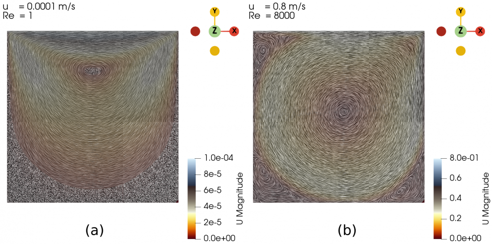
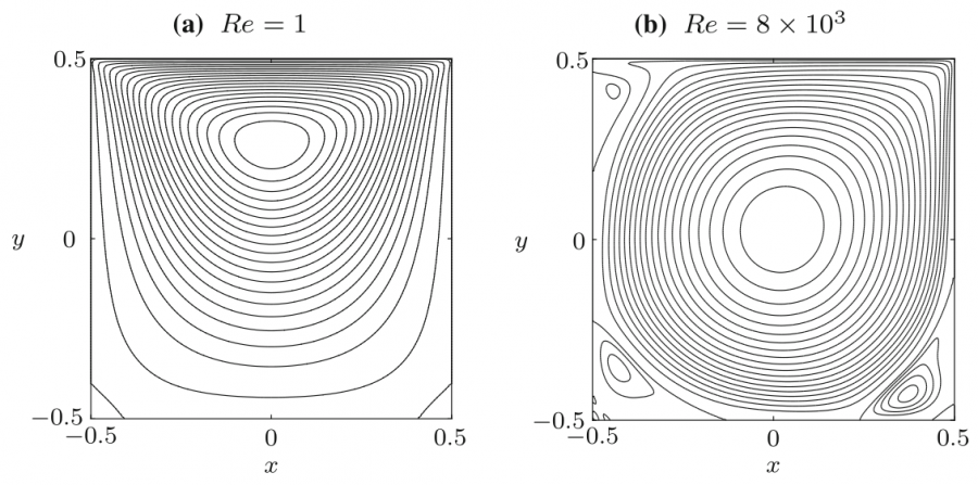
First, we validated our simulation by comparing the case with U = 0.0001 m/s and U = 0.8 m/s, hence the Re are 1 and 8000, respectively, with the case from a study conducted by Hendriketal [1], also with the same Re. The fluid flow with the isolines (streamlines) from both simulation and reference [1] can be seen in the Fig. 1 and Fig. 2 below. It can be seen that the results generated by our simulations is the same as the results obtained from [1].
The flow with Re = 1 is laminar and almost vertically symmetrical and the flow with Re = 8000 is turbulent with 3 secondary eddies in the 3 corners of the cavity.
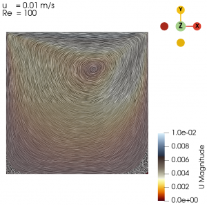
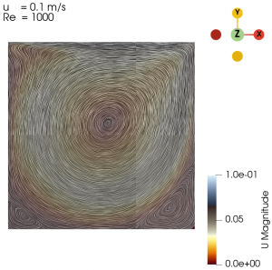
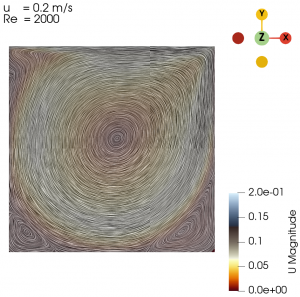
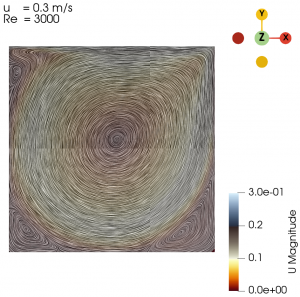
Next we varied the parameter of U from 0.01 m/s to 0.3 m/s with simpleFoam laminar model as per Table 1, and look at the flow profile of the cavity. The isolines can be seen at Fig. 3 to Fig. 10.
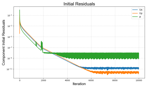
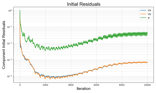
Convergence can be seen from simulation's variables residuals below.
Re = 1
Re = 8000
References:
[1] H. C. Kuhlmann and F. Romanò, "The Lid-Driven Cavity," Computational Methods in Applied Sciences, vol. 50, 2019. https://doi.org/10.1007/978-3-319-91494-7_8
Lid-Driven Cavity with DAI5 Framework
This is a video essay of the application of DAI5 Framework in understanding lid-driven cavity. The lid-driven cavity simulation is done using OpenFOAM.
Disclaimer: the video is in Bahasa Indonesia.
Lid-Driven Cavity Case File: bit.ly/CavityDAI5
Paper Draft
Grid Independency Study on the Turbulence of Lid Driven Cavity using DAI5 Framework
Mid Test with ChatGPT
| Mid Test with ChatGPT | ||
| User | ||
| ChatGPT | ||
| I am going to take an exam on the subject of basic Computational Fluid Dynamics (CFD). I need you to create a basic test consisted of 5 short-answer questions all at once and grade what I do. | ||
| Here’s a basic test on Computational Fluid Dynamics (CFD) consisting of 5 short-answer questions:
Question 1: Define the term "viscosity" and explain its significance in fluid flow. Question 2: What is the difference between laminar and turbulent flow? Provide examples of each. Question 3: Explain the concept of grid independence in CFD and why it is important for accurate simulation results. Question 4: Describe the role of the Navier-Stokes equations in CFD. What do they represent? Question 5: What are boundary conditions in CFD, and why are they crucial for setting up a simulation?
|
||
| 1. Define the term "viscosity" and explain its significance in fluid flow.
Viscosity is a measure of a fluid’s internal friction or resistance to deformation or flow when a force is applied to it. It is a fluid-specific property where fluids with higher viscosity, like syrup, deform less easily compared to fluids with lower viscosity, like water. There are two types of viscosity, the dynamic viscosity (mu) and the kinematic viscosity (nu), with units kg/m.s and m^2/s, respectively. In fluid flow applications, viscosity plays a vital role in determining whether the flow is laminar or turbulent. Viscosity is a critical property that affects fluid dynamics, influencing how fluids flow and behave under various conditions. 2. What is the difference between laminar and turbulent flow? Provide examples of each. Laminar flow is characterized by smooth, orderly motion of fluid layers, with each layer sliding past the adjacent ones with minimal to no mixing. This type of flow typically occurs at low Reynolds numbers (Re < 2000). An example of laminar flow is the flow of blood inside our capillaries or the flow of air inside a wind tunnel before contact. Turbulent flow, on the other hand, is characterized by irregular fluid motion with significant mixing and fluctuations in velocity. This type of flow typically occurs at high Reynolds numbers (Re > 4000). An example of turbulent flow is the air in and out of our respiratory system or the airflow around an airplane wing. 3. Explain the concept of grid independence in CFD and why it is important for accurate simulation results. Grid independence refers to the condition where the results of a simulation do not significantly change with further refinement of the computational grid (mesh). This can be done with a grid dependence study, which is a procedure of successive refinement of an initially coarse grid until certain key results do not change. Achieving grid independence is crucial because it ensures that the numerical solution is not influenced by the discretization of the domain, leading to more reliable and accurate results. A systematic search for grid-independent result forms an essential part of all high-quality CFD studies. 4. Describe the role of the Navier-Stokes equations in CFD. What do they represent? The Navier-Stokes equations are a set of nonlinear partial differential equations that describe the motion of fluid. They represent the conservation of momentum in fluid flow and are fundamental to the field of computational fluid dynamics. The equations account for viscosity, pressure, and external forces acting on the fluid. In CFD, solving the Navier-Stokes equations enables the prediction of velocity fields, pressure distributions, and other flow characteristics, making them essential for simulating and analyzing fluid behavior in various engineering applications. 5. What are boundary conditions in CFD, and why are they crucial for setting up a simulation? Boundary conditions in CFD define the behavior of the fluid at the boundaries of the computational domain. They specify values for variables such as velocity, pressure, and other relevant quantities at the edges of the simulation space. They ensure that the simulation reflects the physical reality of the problem being modeled, allowing for accurate predictions and are essential for producing valid and reliable CFD results. | ||
Grading:
Your explanation is clear and well-structured. You correctly define viscosity and its types (dynamic and kinematic) along with their units. You also mention its importance in fluid dynamics and how it affects flow behavior. One minor note: You could expand on how viscosity affects energy dissipation in the flow. Nonetheless, your answer is quite strong.
Excellent explanation of both laminar and turbulent flows with clear examples and correct references to Reynolds numbers. The distinction between orderly and chaotic motion is well articulated, and the examples are accurate.
Great explanation! You correctly identify grid independence and explain the grid dependence study and its importance in ensuring simulation accuracy. This is a key concept in CFD, and your description captures it thoroughly.
Your answer effectively highlights the significance of the Navier-Stokes equations in CFD. You mention their role in momentum conservation, accounting for viscosity, pressure, and forces, and how they are used to predict key flow characteristics. This is a complete and concise answer.
Good explanation of boundary conditions and their role in simulations. You correctly mention their importance in defining variables at the boundaries and ensuring physical realism in the model. A small suggestion: you could briefly touch upon specific types of boundary conditions (e.g., Dirichlet, Neumann) for more depth, but your answer is still very solid. Overall Score: 96/100 Excellent work! Your understanding of CFD fundamentals is strong, and you provided clear, well-articulated answers throughout the test. Just minor improvements in elaboration could make it even better. |
||
| How does viscosity affects energy dissipation in the fluid flow? Could you elaborate? | ||
| Viscosity affects energy dissipation in fluid flow by resisting the motion of fluid layers, converting kinetic energy into thermal energy (heat) through internal friction. Here’s how this process works in detail:
Internal Friction and Shear Stress: Viscosity causes internal friction between adjacent layers of fluid moving at different velocities. This friction leads to shear stress, which requires energy to maintain. As layers slide past each other, some of the flow’s kinetic energy is “used up” in overcoming this frictional resistance. Conversion of Kinetic Energy to Heat: The energy needed to overcome the viscous forces does not just vanish; it’s transformed into heat. This phenomenon is known as viscous dissipation. In regions with high velocity gradients (such as near solid boundaries in turbulent flows), the energy dissipation rate is higher, causing more kinetic energy to be converted to heat. Impact on Flow Types: Laminar Flow: In low-viscosity, laminar flows, this energy dissipation is relatively low, as the layers slide smoothly over each other. However, viscosity is still crucial for determining the flow regime and ensuring the orderly motion of fluid layers. Turbulent Flow: In turbulent flows, viscosity plays a larger role in dissipating energy. The chaotic, fluctuating motion of fluid particles in turbulence generates numerous small eddies, which further increase the velocity gradients and amplify the energy dissipation through viscous effects. Implications in Engineering and CFD: High-viscosity fluids dissipate more energy as heat, which can be critical for cooling and lubrication applications. In CFD, accurately modeling viscosity is essential to capture realistic energy dissipation, especially in simulations involving turbulent flows, as it affects flow stability, boundary layer characteristics, and even heat transfer predictions. Understanding viscosity's role in energy dissipation is crucial for designing efficient fluid systems, as well as for accurately predicting fluid behavior in simulations. |
||
| What are the Dirichlet and Neumann boundary conditions? What other types of boundary conditions are there? | ||
In CFD, boundary conditions define how fluid behaves at the edges of the simulation domain. Here’s a breakdown of Dirichlet and Neumann boundary conditions, along with a few other common types:
This boundary condition specifies a fixed value for a field variable (like velocity, pressure, or temperature) at the boundary. For instance, setting the temperature on a wall to a constant value (e.g., 300 K) or prescribing a fixed velocity at an inlet. Dirichlet conditions are commonly used to impose known values at inflow boundaries or solid surfaces with a constant temperature.
This condition specifies a fixed rate of change, or gradient, of a variable at the boundary rather than the variable's value itself. For example, setting the heat flux across a wall surface to a constant (which relates to the temperature gradient) or defining a zero-velocity gradient (indicating no shear stress). Neumann conditions are often applied when the exact value is unknown, but the flux or rate of change at the boundary is known, such as insulated walls (zero heat flux) or stress-free outflows.
This combines aspects of Dirichlet and Neumann conditions by defining a relationship between the variable and its gradient at the boundary. For instance, in heat transfer, it can represent convective cooling, where the heat flux is proportional to the temperature difference between the fluid and the boundary (e.g., Newton's Law of Cooling). Robin conditions are used in situations where the boundary value depends on both the internal variable and its rate of change, such as semi-permeable membranes or convective heat transfer.
This boundary condition enforces a repeating pattern in space, where the variables on one side of the boundary match those on the opposite side. For example, in simulations of flow over a regularly spaced array of objects, where the pattern of flow repeats, periodic conditions allow efficient modeling by simulating just a small section. This is especially useful in simulations of channels, waves, and symmetric or repeating systems.
This condition is applied when the domain has a plane of symmetry, where no flow or gradient exists normal to the symmetry plane. The symmetry boundary implies that the normal component of velocity and the normal gradient of scalar variables (like pressure or temperature) are zero. Useful for reducing computational load by only simulating half or a section of a symmetric geometry, like a cylindrical pipe.
Designed for flow exiting the domain, where minimal influence from the boundary on the internal flow is desired. Outflow boundaries often enforce zero gradients or “do-nothing” conditions to allow fluid to exit freely. In external flow problems, like around an airplane, far-field conditions simulate an open, infinite environment where variables gradually return to ambient values as they move away from the body. Each type of boundary condition serves a specific purpose, helping to set up simulations that accurately reflect real physical scenarios. The choice of boundary condition is crucial as it significantly affects simulation stability and results accuracy. |
||
Self-Assessment
I feel like I learned a lot in this CFD Application class. To me, the Navier-Stokes and its numerical solution are substantial in CFD. I can understand more about the concept and theory of CFD and apply them in an analysis. Based on this self-assessment of my performance, I believe I have met the expectations and objectives of the class thus far, which I feel merits a self-assessment score of 92 out of 100.
Post-Mid Test Plan for the Class
It would be nice to know more about the heat transfer aspects of computational fluid dynamics and how to apply it in a case problem.
Computational Fluid Dynamics (CFD) Part 2
Temperature-Difference-Driven Cavity
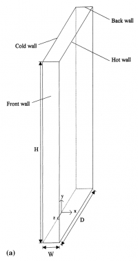
We try to replicate the study conducted by Betts and Bokhari. Here, we have a rectangular cavity with the dimensions of 0.076 m x 0.52 m x 2.18 m in the x, y, and z axis, respectively, as seen in the figure below. There are no lids in this cavity. Rather, the cavity is driven by temperature difference. The right wall is constantly heated to 39.9 °C, while the left wall is constantly heated to 19.6 °C.
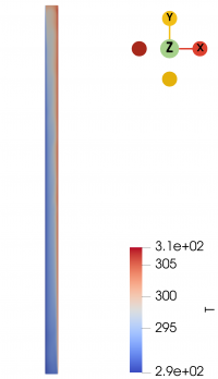
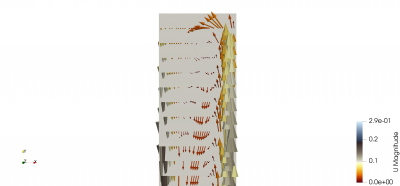
The objective of this study is to understand the fluid flow (in this case, air) due to the temperature difference. The assumptions are the flow is in steady-state. The study is done using OpenFOAM with buoyantSimpleFoam solver with kOmegaSST turbulence model. Rather than specifying the velocity in the boundary condition, the case will have temperature in the boundary condition. The case file can be downloaded from buoyantCavity
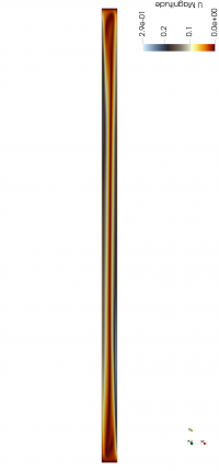
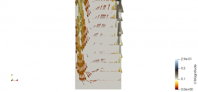
It can be seen from the 2 images above that there exist a temperature difference on the right and left walls. This temperature difference lead to the flow of the air inside the cavity. The flow of the air inside the cavity resembles the elongated vortex that can be seen more detailed in the zoomed-in images below.
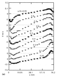
If we look at the velocity profile in the y axis direction in the centerline of the cavity, we can be certain that there exist a vortex inside the cavity. The velocity profile can be seen in the images below, with a close comparison to the study conducted by Betts and Bokhari.
Reference: P.L. Betts, I.H. Bokhari, "Experiments on turbulent natural convection in an enclosed tall cavity," International Journal of Heat and Fluid Flow, vol. 21, pp. 675-683, 2000.
Lid-Driven Cavity with Artificial Neural Network (ANN)
Using the data from the previous study Cavity 2D with OpenFOAM, we gather 4 variations of lid velocity of the cavity, 0.01, 0.05, 0.1, 0.3 m/s. With this 4 variations of velocity, along with the x and y coordinates of the cells of the control volume of the 50x50 grid cavity (the mesh cells), we can gather the 10,000 rows of data as the input for the ANN modeling with the pressure (p), x-axis velocity component (Ux), and y-axis velocity component (Uy) in said coordinate as the output of the ANN modeling.
The simulation files, the input-output table, and the Python codes can be downloaded here.
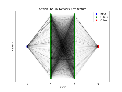
From the ANN modeling with 2 hidden layers and 128 neurons per hidden layer, as seen in the ANN Architecture below, and 500 epochs, it can be seen that the evaluation of the model yields relatively good results.
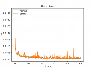
The ANN modeling resulted in the model loss of less than 5e-4 as seen below.
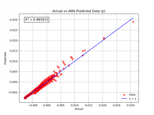
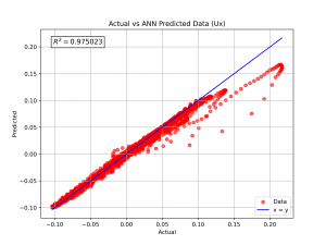
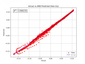
The ANN model can predict the p, Ux, and Uy with coefficient of determination (R²) of more than 0.985, 0.975, and 0.99, respectively, as seen below.
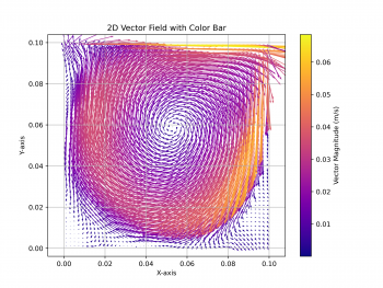
This is further supported by the visualization of the airflow inside the cavity. Here, we compare the velocity vector field of lid-driven cavity with the lid moving at 0.1 m/s, both the simulation (actual data) and the ANN prediction (predicted data)
This result can of course be improved by varying the ANN modeling parameters such as the number of hidden layer, the number of neurons per hidden layer, and the number of epoch, and also adding more and more data from the variations of simulation to cover a broader range of conditions.
Discussion with ChatGPT: Continuum Mechanics
| Continuum Mechanics | ||
| USER | ||
| AI | ||
| Can you give a practical example (along with a simple calculator for a 1D problem) in engineering where continuum mechanics treats materials as continuous, focusing on the integration of an uninterrupted 'conscious continuum' into the DAI5 framework. | ||
| Certainly! Continuum mechanics simplifies the study of materials by assuming they are continuous and devoid of voids, even though materials are composed of discrete particles. This assumption allows engineers to use mathematical tools, such as differential equations and integration, to analyze stresses, strains, and material behavior. Let’s create a practical example in engineering:
Problem: 1D Axial Deformation of a Rod A steel rod of length L=1.0m, cross-sectional area A=0.01m², and Young's modulus E=200GPa is subjected to a tensile force F=10,000N. The goal is to calculate the elongation ΔL of the rod using continuum mechanics and integrate it with the DAI5 framework as an uninterrupted "conscious continuum." Continuum Mechanics Solution: Using the 1D axial deformation formula: ΔL=FL/AE where F = Applied force, L = Original length, A = Cross-sectional area, E = Young's modulus DAI5 Framework Integration: Intention: Understand how a tensile force deforms a continuous rod in 1D. Initial Thinking: Assume a linear elastic behavior where stress and strain follow Hooke's Law. Define the rod as a continuum, ignoring atomic-scale irregularities. Idealization: Use the governing equation derived from Hooke’s Law, treating material properties as constant and uniformly distributed. Instruction Set: Write a program to calculate the elongation and visualize its dependence on F, A, E, and L.
F = 10000 # Force in Newtons L = 1.0 # Length in meters A = 0.01 # Cross-sectional area in square meters E = 200e9 # Young's modulus in Pascals delta_L = (F * L) / (A * E) print(f"Elongation (ΔL): {delta_L:.6f} m") |
||
Reduced-Order Model (ROM) using Python: 1D Conduction
In Progress.
Reduced-Order Model (ROM) using ITHACA-FV: Backward Facing Step (PitzDaily)
In Progress.
(EOF)
