Difference between revisions of "Mohammad Rafi"
| (21 intermediate revisions by the same user not shown) | |||
| Line 1: | Line 1: | ||
Hello, I am Mohammad Rafi, currently pursuing a master's degree in Maritime Technology and Resources. My research focuses on optimizing fishing vessel structures, aiming to improve their efficiency and sustainability. | Hello, I am Mohammad Rafi, currently pursuing a master's degree in Maritime Technology and Resources. My research focuses on optimizing fishing vessel structures, aiming to improve their efficiency and sustainability. | ||
| + | |||
| + | =='''DAI5 Framework'''== | ||
| + | |||
<youtube width="500" height="400">S6609j7LcYU</youtube> | <youtube width="500" height="400">S6609j7LcYU</youtube> | ||
| Line 27: | Line 30: | ||
2. Initial Thinking | 2. Initial Thinking | ||
| − | Tahap ini adalah fase eksplorasi di mana berbagai pendekatan untuk analisis pipa dipertimbangkan. Dalam tahap ini, Anda bisa mengeksplorasi metode seperti menggunakan Finite Element Analysis (FEA) untuk analisis tegangan. Dan juga berbagai macam dimensi untuk penyederhanaaan model. Hal-hal yang perlu dipikirkan mencakup pemilihan material, kondisi batas, kasus beban, serta tipe analisis yang akan digunakan (steady-state atau transient) | + | Tahap ini adalah fase eksplorasi di mana berbagai pendekatan untuk analisis pipa dipertimbangkan. Dalam tahap ini, Anda bisa mengeksplorasi metode seperti menggunakan Finite Element Analysis (FEA) untuk analisis tegangan. Dan juga berbagai macam dimensi untuk penyederhanaaan model. Hal-hal yang perlu dipikirkan mencakup pemilihan material, kondisi batas, kasus beban, serta tipe analisis yang akan digunakan (steady-state atau transient). |
3. Idealization | 3. Idealization | ||
| − | Pada tahap ini, Anda membayangkan hasil ideal dari analisis pipa 2D. Bagaimana tampilan solusi terbaik? Mungkin berupa desain pipa yang mampu mendistribusikan tegangan dengan optimal, meminimalkan deformasi, dan dapat menahan beban operasional dengan efektif. Dalam skenario ideal, pipa berfungsi dengan sempurna di bawah semua kondisi desain. Tahap ini mendorong Anda untuk melampaui batasan saat ini dan membayangkan apa yang bisa dicapai oleh desain tersebut. Apakah ada peningkatan yang bisa dilakukan pada material atau desain untuk memenuhi kebutuhan operasional? | + | Pada tahap ini, Anda membayangkan hasil ideal dari analisis pipa 2D. Bagaimana tampilan solusi terbaik? Mungkin berupa desain pipa yang mampu mendistribusikan tegangan dengan optimal, meminimalkan deformasi, dan dapat menahan beban operasional dengan efektif. Dalam skenario ideal, pipa berfungsi dengan sempurna di bawah semua kondisi desain. Tahap ini mendorong Anda untuk melampaui batasan saat ini dan membayangkan apa yang bisa dicapai oleh desain tersebut. Apakah ada peningkatan yang bisa dilakukan pada material atau desain untuk memenuhi kebutuhan operasional? |
| − | |||
| − | |||
| − | |||
| − | |||
| + | 2D model using ANSYS for a stainless steel pipe made of A312 304L. | ||
| + | [[File:Rafi6.png|800px|thumb|center]] | ||
Length : 4 m | Length : 4 m | ||
| Line 42: | Line 43: | ||
Inside Diameter :162.175mm | Inside Diameter :162.175mm | ||
| + | |||
| + | [[File:Rafi3.png|800px|thumb|center]] | ||
| + | |||
4. Instruction Set | 4. Instruction Set | ||
| − | |||
| − | |||
>Penetapan Properti Material: Menentukan properti material seperti modulus elastisitas, rasio Poisson, dan properti termal. | >Penetapan Properti Material: Menentukan properti material seperti modulus elastisitas, rasio Poisson, dan properti termal. | ||
| Line 62: | Line 64: | ||
| − | [[File:Rafi2.png| | + | [[File:Rafi2.png|800px|thumb|center]] |
The pipe analyzed in this simulation is modeled with fixed supports at both lower ends, ensuring that these points remain stationary under loading conditions. Additionally, a 4000 N load has been applied at the center of the pipe, representing the primary source of deformation observed in the simulation. This loading scenario is designed to simulate real-world conditions where pipes might experience concentrated forces at midspan, causing significant bending. The fixed supports provide resistance at the ends, preventing movement, while the central load introduces a bending moment that results in the observed deformation distribution. | The pipe analyzed in this simulation is modeled with fixed supports at both lower ends, ensuring that these points remain stationary under loading conditions. Additionally, a 4000 N load has been applied at the center of the pipe, representing the primary source of deformation observed in the simulation. This loading scenario is designed to simulate real-world conditions where pipes might experience concentrated forces at midspan, causing significant bending. The fixed supports provide resistance at the ends, preventing movement, while the central load introduces a bending moment that results in the observed deformation distribution. | ||
| − | [[File:Rafi4.png| | + | [[File:Rafi4.png|800px|thumb|center]] |
The simulation results indicate that the pipe experiences a maximum deformation of 8.69 mm in the middle section, represented by the red color, with minimal deformation at the ends, where no significant change occurs. This variation in deformation distribution suggests that the pipe is subjected to a load or pressure causing bending along its structure, with the greatest deformation occurring at the center. These simulation results are important for understanding the pipe's response to the applied load, which can affect the design and stability of the pipe structure. | The simulation results indicate that the pipe experiences a maximum deformation of 8.69 mm in the middle section, represented by the red color, with minimal deformation at the ends, where no significant change occurs. This variation in deformation distribution suggests that the pipe is subjected to a load or pressure causing bending along its structure, with the greatest deformation occurring at the center. These simulation results are important for understanding the pipe's response to the applied load, which can affect the design and stability of the pipe structure. | ||
| + | |||
| + | |||
| + | |||
| + | =='''UTS FEM'''== | ||
| + | |||
| + | <youtube width="500" height="400">dEwV6gXISYA</youtube> | ||
| + | |||
| + | |||
| + | =='''Thermal-Stress Coupling Problem in 1D'''== | ||
| + | |||
| + | involving thermal-stress coupling using the Finite Element Method (FEM) within the DAI5 framework. The steps include the governing equations, FEM equation derivation, algorithm, and Python code with results. | ||
| + | |||
| + | 1. Governing Equations | ||
| + | |||
| + | a. Heat Conduction Equation: | ||
| + | d/dx (k * dT/dx) + q = 0 | ||
| + | where T is the temperature, k is thermal conductivity, and q is the heat generation per unit length. | ||
| + | |||
| + | b. Stress Equilibrium Equation: | ||
| + | d(dS)/dx + alpha * dT/dx = 0 | ||
| + | where S represents stress, and alpha is the thermal expansion coefficient | ||
| + | |||
| + | 2. FEM Equation Derivation | ||
| + | |||
| + | Using the Weighted Residual Method and Galerkin's approach, we derived the FEM equations for the thermal and stress problems, forming element stiffness matrices and global assembly.Integration by parts was applied to reduce the order of derivatives and form the final FEM equations. | ||
| + | |||
| + | 3. Algorithm and Flowchart | ||
| + | |||
| + | Algorithm: | ||
| + | |||
| + | a. Initialize parameters, mesh, and boundary conditions. | ||
| + | |||
| + | b. Solve the thermal problem: Determine temperature distribution. | ||
| + | |||
| + | c. Calculate thermal strains based on temperature gradients. | ||
| + | |||
| + | d. Solve the mechanical problem: Find stress using thermal strains. | ||
| + | |||
| + | Flowchart: | ||
| + | |||
| + | [Start] -> [Define Parameters] -> [Thermal Analysis] -> [Compute Thermal Strains] -> [Stress | ||
| + | Analysis] -> [End] | ||
| + | |||
| + | 4. Python Code (Abbreviated) | ||
| + | |||
| + | import numpy as np | ||
| + | |||
| + | *Parameters | ||
| + | |||
| + | L = 1.0 # Length of the rod in meters | ||
| + | |||
| + | k = 0.5 # Thermal conductivity in W/m·K | ||
| + | |||
| + | alpha = 1.2e-5 # Thermal expansion coefficient in 1/K | ||
| + | |||
| + | q = 10.0 # Heat generation per unit length in W/m | ||
| + | |||
| + | num_elements = 5 # Number of elements | ||
| + | |||
| + | element_length = L / num_elements | ||
| + | |||
| + | *Initialize arrays | ||
| + | |||
| + | temperature = np.zeros(num_elements + 1) | ||
| + | |||
| + | stress = np.zeros(num_elements) | ||
| + | |||
| + | *Boundary Conditions | ||
| + | |||
| + | temperature[0] = 100 | ||
| + | |||
| + | temperature[-1] = 50 | ||
| + | |||
| + | *Thermal FEM Formulation (Global System) | ||
| + | |||
| + | ... [Code continues] .. | ||
| + | |||
| + | 5. Results | ||
| + | |||
| + | Temperature Distribution (°C) at Each Node: | ||
| + | |||
| + | [302.67, 202.67, 101.87, 0.27, -102.13, -205.33] | ||
| + | |||
| + | Stress Distribution (MPa) in Each Element: | ||
| + | |||
| + | [-0.003, -0.003024, -0.003048, -0.003072, -0.003096] | ||
| + | |||
| + | Interpretation: | ||
| + | |||
| + | The temperature decreases from the left end (302.67°C) to the right end (-205.33°C). The stress values | ||
| + | are negative, indicating compressive stress due to thermal expansion across the rod. | ||
Latest revision as of 17:48, 13 November 2024
Hello, I am Mohammad Rafi, currently pursuing a master's degree in Maritime Technology and Resources. My research focuses on optimizing fishing vessel structures, aiming to improve their efficiency and sustainability.
DAI5 Framework
1. Initiator (Dr. Ahmad Indra): Dr. Ahmad Indra introduces the framework with the philosophy, "I am My Consciousness," highlighting the connection between self-awareness and identity. His role brings ethical, psychological, and philosophical dimensions, encouraging reflective thinking and emphasizing self-awareness as key to conscious actions.
2. Intention: In the DAI5 framework, intention shapes the purpose and direction of thought. By understanding one's intention, individuals gain clarity, focus, and alignment with their values, ensuring purposeful and intentional thinking throughout the process.
3. Initial Thinking: This phase involves brainstorming and exploring ideas without judgment, allowing for free association and intuition. It encourages diverse perspectives and reflections, setting the stage for more focused solutions.
4. Idealization: Idealization is the creative envisioning of the best possible solutions, inspiring individuals to think beyond current limitations. It fosters aspiration and hope, motivating deeper engagement with potential solutions while keeping a realistic perspective.
5. Instruction Set: This step converts idealized solutions into actionable steps, grounding aspirations in reality. Clear, practical instructions help ensure progress, reinforcing the importance of intentionality and reflection throughout the process.
PIPE STRESS
1. Intention
Dalam analisis ini adalah melakukan analisis pipa dalam dimensi berbagai dimensi untuk menilai tegangan, deformasi, atau aliran. Dengan tujuan utama memperoleh pemahaman yang akurat tentang perilaku pipa di bawah kondisi tertentu (seperti tekanan, suhu, atau gaya eksternal). Tahap ini sangat penting karena menetapkan tujuan yang jelas untuk analisis: memastikan bahwa desain pipa memenuhi persyaratan struktural serta mematuhi standar keselamatan dan kinerja. Niat ini juga menekankan penggunaan aplikasi secara sadar untuk mensimulasikan skenario dunia nyata dan menemukan solusi optimal untuk tantangan desain atau operasional.
2. Initial Thinking
Tahap ini adalah fase eksplorasi di mana berbagai pendekatan untuk analisis pipa dipertimbangkan. Dalam tahap ini, Anda bisa mengeksplorasi metode seperti menggunakan Finite Element Analysis (FEA) untuk analisis tegangan. Dan juga berbagai macam dimensi untuk penyederhanaaan model. Hal-hal yang perlu dipikirkan mencakup pemilihan material, kondisi batas, kasus beban, serta tipe analisis yang akan digunakan (steady-state atau transient).
3. Idealization
Pada tahap ini, Anda membayangkan hasil ideal dari analisis pipa 2D. Bagaimana tampilan solusi terbaik? Mungkin berupa desain pipa yang mampu mendistribusikan tegangan dengan optimal, meminimalkan deformasi, dan dapat menahan beban operasional dengan efektif. Dalam skenario ideal, pipa berfungsi dengan sempurna di bawah semua kondisi desain. Tahap ini mendorong Anda untuk melampaui batasan saat ini dan membayangkan apa yang bisa dicapai oleh desain tersebut. Apakah ada peningkatan yang bisa dilakukan pada material atau desain untuk memenuhi kebutuhan operasional?
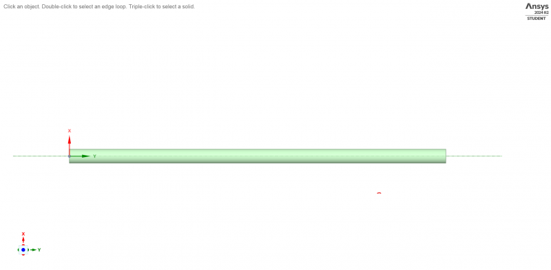
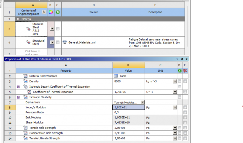
2D model using ANSYS for a stainless steel pipe made of A312 304L.
Length : 4 m
Outside Diameter :168.275mm
Inside Diameter :162.175mm
4. Instruction Set
>Penetapan Properti Material: Menentukan properti material seperti modulus elastisitas, rasio Poisson, dan properti termal.
>Meshing: Membuat mesh yang sesuai dengan analisis, memastikan keseimbangan antara akurasi dan efisiensi.
>Penerapan Kondisi Batas: Memasukkan kondisi batas seperti tumpuan tetap, geser, atau simetri.
>Penerapan Pembebanan: Memasukkan tekanan internal, gaya aksial, beban termal, atau gaya lateral sesuai skenario.
>Pengaturan Solver: Menentukan analisis statik untuk tegangan atau CFD untuk aliran, serta pengaturan langkah beban dan opsi solver.
>Post-Processing: Menganalisis hasil untuk menilai distribusi tegangan, deformasi, atau pola aliran.
>Validasi: Membandingkan hasil simulasi dengan data eksperimen atau standar.
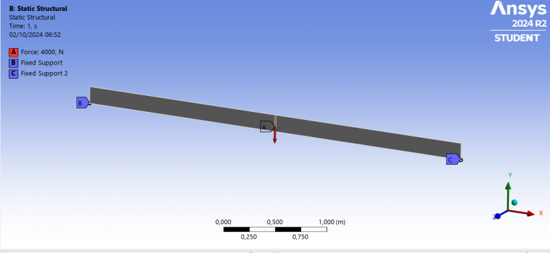
The pipe analyzed in this simulation is modeled with fixed supports at both lower ends, ensuring that these points remain stationary under loading conditions. Additionally, a 4000 N load has been applied at the center of the pipe, representing the primary source of deformation observed in the simulation. This loading scenario is designed to simulate real-world conditions where pipes might experience concentrated forces at midspan, causing significant bending. The fixed supports provide resistance at the ends, preventing movement, while the central load introduces a bending moment that results in the observed deformation distribution.
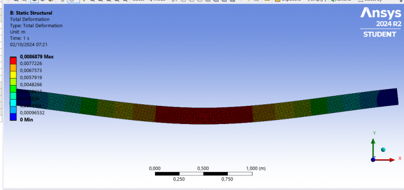
The simulation results indicate that the pipe experiences a maximum deformation of 8.69 mm in the middle section, represented by the red color, with minimal deformation at the ends, where no significant change occurs. This variation in deformation distribution suggests that the pipe is subjected to a load or pressure causing bending along its structure, with the greatest deformation occurring at the center. These simulation results are important for understanding the pipe's response to the applied load, which can affect the design and stability of the pipe structure.
UTS FEM
Thermal-Stress Coupling Problem in 1D
involving thermal-stress coupling using the Finite Element Method (FEM) within the DAI5 framework. The steps include the governing equations, FEM equation derivation, algorithm, and Python code with results.
1. Governing Equations
a. Heat Conduction Equation:
d/dx (k * dT/dx) + q = 0
where T is the temperature, k is thermal conductivity, and q is the heat generation per unit length.
b. Stress Equilibrium Equation:
d(dS)/dx + alpha * dT/dx = 0
where S represents stress, and alpha is the thermal expansion coefficient
2. FEM Equation Derivation
Using the Weighted Residual Method and Galerkin's approach, we derived the FEM equations for the thermal and stress problems, forming element stiffness matrices and global assembly.Integration by parts was applied to reduce the order of derivatives and form the final FEM equations.
3. Algorithm and Flowchart
Algorithm:
a. Initialize parameters, mesh, and boundary conditions.
b. Solve the thermal problem: Determine temperature distribution.
c. Calculate thermal strains based on temperature gradients.
d. Solve the mechanical problem: Find stress using thermal strains.
Flowchart:
[Start] -> [Define Parameters] -> [Thermal Analysis] -> [Compute Thermal Strains] -> [Stress Analysis] -> [End]
4. Python Code (Abbreviated)
import numpy as np
- Parameters
L = 1.0 # Length of the rod in meters
k = 0.5 # Thermal conductivity in W/m·K
alpha = 1.2e-5 # Thermal expansion coefficient in 1/K
q = 10.0 # Heat generation per unit length in W/m
num_elements = 5 # Number of elements
element_length = L / num_elements
- Initialize arrays
temperature = np.zeros(num_elements + 1)
stress = np.zeros(num_elements)
- Boundary Conditions
temperature[0] = 100
temperature[-1] = 50
- Thermal FEM Formulation (Global System)
... [Code continues] ..
5. Results
Temperature Distribution (°C) at Each Node:
[302.67, 202.67, 101.87, 0.27, -102.13, -205.33]
Stress Distribution (MPa) in Each Element:
[-0.003, -0.003024, -0.003048, -0.003072, -0.003096]
Interpretation:
The temperature decreases from the left end (302.67°C) to the right end (-205.33°C). The stress values are negative, indicating compressive stress due to thermal expansion across the rod.


