Difference between revisions of "Dzakiyya Yumna Fitrasani"
(→Final Case Study Report) |
(→Introduction) |
||
| Line 2: | Line 2: | ||
== Introduction == | == Introduction == | ||
| − | |||
Hello, my name is '''Dzakiyya'''. I am a student in '''Metode Numerik-01'''. This will be my page regarding Metode Numerik. | Hello, my name is '''Dzakiyya'''. I am a student in '''Metode Numerik-01'''. This will be my page regarding Metode Numerik. | ||
Latest revision as of 18:56, 27 July 2024
Contents
[hide]Introduction
Hello, my name is Dzakiyya. I am a student in Metode Numerik-01. This will be my page regarding Metode Numerik.
FULLNAME: Dzakiyya Yumna Fitrasani
STUDENT NUMBER: 2106728055
Numerical Methods in Mechanical Engineering / 22 May 2023
Numerical methods are extensively used in various areas of mechanical engineering to solve complex mathematical equations, simulate physical phenomena, and optimize designs. Here are some applications of numerical methods in mechanical engineering:
1. Solving Equations: Numerical methods such as root-finding algorithms (e.g., Newton-Raphson method) and numerical integration techniques (e.g., Simpson's rule, trapezoidal rule) are used to solve equations encountered in mechanical engineering, such as finding the roots of nonlinear equations or evaluating integrals in engineering analysis.
2. Finite Element Analysis (FEA): FEA is widely used in mechanical engineering for structural analysis. It involves dividing a complex structure into smaller finite elements and solving the equations of equilibrium numerically. FEA helps in determining stress, strain, deformation, and failure criteria in mechanical components and systems. It is used in the design and optimization of structures, such as buildings, bridges, and machine components.
3. Computational Fluid Dynamics (CFD): CFD is employed to analyze fluid flow and heat transfer in mechanical systems. Numerical methods, such as finite volume or finite element methods, are used to discretize the fluid domain and solve the governing equations (e.g., Navier-Stokes equations). CFD is applied in the design of aerodynamic profiles, HVAC systems, combustion chambers, and optimization of fluid flow in pipes and channels.
4. Optimization and Design: Numerical optimization techniques, such as genetic algorithms, gradient-based methods, and response surface methods, are employed to optimize designs in mechanical engineering. These methods help in finding optimal solutions for parameters like shape, size, material selection, and operating conditions, considering constraints and objective functions.
These are just a few examples of how numerical methods are applied in mechanical engineering. These methods enable engineers to solve complex problems, make informed design decisions, optimize performance, and reduce the need for costly physical experiments.
Hydrogen Storage Design, Optimization, and Calculation
A. Hydrogen storage technologies
Storing hydrogen in gaseous form requires two main components – a storage compartment and a compressor to achieve higher storage pressure and increase the storage density. Gaseous hydrogen is usually not stored in pressure exceeding 100 bar in vessels above ground and 200 bar for underground storage (Wolf, 2015). The low density of hydrogen leads to the requirement of large storage volumes, and as a consequence, usually large investment costs. However, higher pressure e.g. 700 bar requires advanced vessel materials such as carbon fiber, which makes it very expensive and not considered viable for large-scale applications (Andersson & Grönkvist, 2019). One of the main advantages of storing hydrogen as compressed gas compared to liquid hydrogen is that most applications for hydrogen today require hydrogen in gaseous form.
B. Aspects to be considered in designing hydrogen storage
When designing hydrogen storage systems, several aspects need to be considered to ensure safety, efficiency, and practicality. Here are some factors to take into account:
1. Material Compatibility: Hydrogen can interact with various materials, leading to embrittlement or leakage. It is essential to select materials that are compatible with hydrogen and can withstand the operating conditions of the storage system. This includes considering factors such as material strength, corrosion resistance, and permeability to hydrogen.
2. Cost: The cost of the storage system plays a significant role in its viability. Design considerations should focus on optimizing cost-effectiveness while meeting the required storage capacity and safety standards.
3. Safety: Hydrogen is highly flammable and has a wide flammability range, so safety is of utmost importance. Storage systems must be designed to minimize the risk of leaks, explosions, and other hazards. Safety measures may include using robust materials, incorporating pressure relief devices, implementing proper ventilation, and ensuring effective leak detection systems.
4. Efficiency: The storage system should minimize energy losses during storage and retrieval processes. Any energy required for compression should be considered. Additionally, the system should minimize energy losses due to heat transfer or leakage.
5. Regulations and Standards: Compliance with relevant regulations, codes, and standards is crucial to ensure safety and performance. Design considerations should align with existing guidelines or actively contribute to the development of new standards as the hydrogen industry evolves.
C. Hydrogen storage design
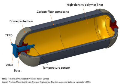
Material: Polymer liner and a composite wrapping
Two types of liners have been produced by rotational molding using the same LLDPE/HDPE blend, the Ø72 x 270 mm (diameter length) prototype liner with an inner volume of 1 L and the actual-scale liner (Ø224 x 725 mm), with an inner volume of 22 L. Fig. 2 shows schematic drawings of both liners.
The fiber-resin composite, with 60% fiber by volume, has a manufactured-listed tensile strength of 2550 MPa.
A fiber winding angle of 15 was used for the helical layers, while angles close to 90 were used for the hoop layers. To help squeeze out excessive resin during the winding process, the helical and hoop layers were wound alternately over the liner.
D. Capacity constraints and optimization
import numpy as np
from scipy.optimize import minimize
def objective(x):
    r, l = x
    volume = np.pi * r**2 * l
    return abs(volume - 1000)  # Target volume is 1000 cubic centimeters (1 liter)
def constraint(x):
    r, l = x
    return [
        r - 36,  # Maximum radius constraint: r <= 36 mm
        l - 270  # Maximum length constraint: h <= 270 mm
    ]
# Initial guess for the radius and length
x0 = [0, 0]
# Define the bounds for the radius and length
bounds = [(0, 36), (0, 270)]
# Define the constraints
constraints = {'type': 'ineq', 'fun': constraint}
# Solve the optimization problem
result = minimize(objective, x0, bounds=bounds, constraints=constraints)
# Print the optimized radius and height
opt_radius, opt_length = result.x
print(f"Optimized radius: {opt_radius} mm")
print(f"Optimized length: {opt_length} mm")
Optimized radius: 35.99999999569217 mm
Optimized length: 269.9999999674908 mm
E. Analysis
Composite wrapping analysis
- Netting analysis
Netting analysis is a preliminary sizing step to estimate the thicknesses of the helical and hoop layers for given pressure load, safety factor, and composite strength.
- Hoop winding angle
The helical and hoop thicknesses are 18.5 mm and 19.6 mm, respectively. The total composite weight of the tank is 107.4 kg.
- L/D ratio
Tanks that fit within the available space onboard a vehicle typically have length-to-diameter ratio between ~1.5 and ~4.0. The results of the analysis showed only a small difference in the amount of composite needed, 103.6 kg for L/D of 1.5 versus 102.0 kg for L/D of 3.0.
- FE liner analysis
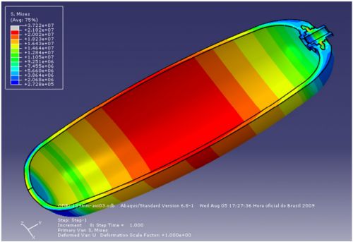
Table 3 shows the variation of the numerical von Mises stress in the central region of the actual liner, for distinct thicknesses, when the simulated maximum hydrostatic pressure is reached. It can be observed that, in all cases, von Mises stress varies within 20–21 MPa.
Fig. 4 shows the distribution of von Mises stress for the actual liner (thickness: 13.9 mm) and it is possible to verify that the central section of the liner is the weakest region. Also, the burst pressure (1.84 MPa) was very close to the experimental burst pressure obtained (1.86 MPa), as shown in Table 3. The same was found for the 12.5 mm-thick liner, but the 9.5 mm and the 15.3 mm-thick liners showed poorer agreement (18% and 17% error, respectively).
Analysis was carried out considering the Tsai-Wu failure criterion and the chosen inner pressure was 20.7 MPa, with a safety factor of 2.0. Fig. 5a and b present the results of the FEA simulation for 40.0 MPa inner liner pressure. The lowest strength ratio was 1.039. This critical condition occurred at the ply#2 of sub laminate 1, and the largest elongation was found at the bottom dome (3.053 mm).
Stress analysis coding
import math
import numpy as np
import matplotlib.pyplot as plt
sig_x = 34.5
sig_y = 70
tau_xy = 43.2
theta_d = 30
theta = theta_d*math.pi/180
# Stresses on an element orientated at theta degrees
sig_x1 = 0.5*(sig_x+sig_y) + 0.5*(sig_x-sig_y)*np.cos(2*theta) + tau_xy*np.sin(2*theta)
sig_y1 = 0.5*(sig_x+sig_y) - 0.5*(sig_x-sig_y)*np.cos(2*theta) - tau_xy*np.sin(2*theta)
tau_x1y1 = -0.5*(sig_x-sig_y)*np.sin(2*theta) + tau_xy*(np.cos(2*theta))
print('(i) Stresses on an element orientated at {one} theta degrees'.format(one=theta_d))
print('— sig_x1 = {one} N/mm^2'.format(one=round(sig_x1,1)))
print('— sig_y1 = {one} N/mm^2'.format(one=round(sig_y1,1)))
print('— tau_x1y1 = {one} N/mm^2'.format(one=round(tau_x1y1,1)))
# Principal planes
theta_1 = 0.5*math.atan((2*tau_xy)/(sig_x-sig_y))
theta_2 = theta_1 + (math.pi/2)
theta_1d = theta_1*(180/math.pi)
theta_2d = theta_2*(180/math.pi)
print('\n')
print('(ii) Principal angles')
print('— The principal angles are {one} and {two} degrees'.format(one=round(theta_1d,1),two=round(theta_2d,1)))
# Principal stresses
sig_1 = 0.5*(sig_x+sig_y) + 0.5*(sig_x-sig_y)*np.cos(2*theta_1) + tau_xy*np.sin(2*theta_1)
sig_2 = 0.5*(sig_x+sig_y) + 0.5*(sig_x-sig_y)*np.cos(2*theta_2) + tau_xy*np.sin(2*theta_2)
print('\n')
print('(iii) Principal stresses')
print('— The principal stresses are {one} N/mm^2 occurs on a plane orientatated at {two} degrees'.format(one=round(sig_1,1), two=round(theta_1d,1)))
print('— The principal stresses are {one} N/mm^2 occurs on a plane orientatated at {two} degrees'.format(one=round(sig_2,1), two=round(theta_2d,1)))
if(sig_1>sig_2):
  print('— sig_1 is {one} N/mm^2 and theta_p1 is {two} degrees'.format(one=round(sig_1,1),two=round(theta_1d)))
  print('— sig_2 is {one} N/mm^2 and theta_p2 is {two} degrees'.format(one=round(sig_2,1),two=round(theta_2d)))
else:
  print('— sig_1 is {one} N/mm^2 and theta_p1 is {two} degrees'.format(one=round(sig_2,1),two=round(theta_2d)))
  print('— sig_2 is {one} N/mm^2 and theta_p2 is {two} degrees'.format(one=round(sig_1,1),two=round(theta_1d)))
# Planes of max +ve/-ve shear stress
if(sig_1>sig_2):
  theta_s1 = theta_1d-45 # Plane for maximum positive shear stress
else:
  theta_s1 = theta_2d-45 # Plane for maximum positive shear stress
theta_s2 = theta_s1+90 # Plane of maximum negative shear stress
print('\n')
print('(iv) Planes of max +ve/-ve shear stress')
print('— Max +ve shear stress occurs on a plane at {one} degrees'.format(one=round(theta_s1,1)))
print('— Max -ve shear stress occurs on a plane at {one} degrees'.format(one=round(theta_s2,1)))
# Maximum shear stress
tau_max = abs(0.5*(sig_2-sig_1))
sig_s = 0.5*(sig_x+sig_y)
print('\n')
print('(v) Maximum shear stress')
print('— The maximum shear stress has a magnitude of {one} N/mm^2'.format(one=round(tau_max,1)))
print('— The normal stress on the max shear stress planes is {one} N/mm^2'.format(one=round(sig_s,1)))
# Plotting
Theta = np.arange(-180,181) #(degrees) Range of angles in degrees
Theta_rad = math.pi/180*Theta #(radians) Convert angles to radians
#Transformation equations
Sig_x1 = 0.5*(sig_x+sig_y) + 0.5*(sig_x-sig_y)*np.cos(2*Theta_rad) + tau_xy*np.sin(2*Theta_rad)
Sig_y1 = 0.5*(sig_x+sig_y) - 0.5*(sig_x-sig_y)*np.cos(2*Theta_rad) - tau_xy*np.sin(2*Theta_rad)
Tau_x1y1 = -0.5*(sig_x-sig_y)*np.sin(2*Theta_rad) + tau_xy*(np.cos(2*Theta_rad))
fig = plt.figure()
axes = fig.add_axes([0.1,0.1,2,1])
# Plot transformation equations
axes.plot(Theta,Sig_x1,'royalblue',label="Normal Stress, $\sigma_x$")
axes.plot(Theta,Sig_y1,'seagreen',label="Normal Stress, $\sigma_y$")
axes.plot(Theta,Tau_x1y1,'lightcoral',label="Shear Stress, $t\_{x1y1}$")
# Plot stresses at 30 degrees
axes.plot([theta_d,theta_d],[sig_x1,sig_y1],'r',linestyle='--',lw=2) # Vertical guide line at 30 degrees
axes.plot([theta_d],[sig_x1],'o',color='lime',markersize=5) # Stress sig_x1
axes.plot([theta_d],[sig_y1],'o',color='lime',markersize=5) # Stress sig_y1
axes.plot([theta_d],[tau_x1y1],'o',color='lime',markersize=5) # Shear tau_x1y1
# Housekeeping
axes.set_xlabel('Angle of face (degrees)')
axes.set_ylabel('Stress $(N/mm^2)$')
axes.set_title('Stress variation with angle')
axes.set_xlim([-180,180])
axes.set_xticks(np.arange(-180,180,20))
axes.legend(loc='lower left')
print('\n')
print('(vi) Plotting')
plt.grid()
plt.show()
(i) Stresses on an element orientated at 30 theta degrees
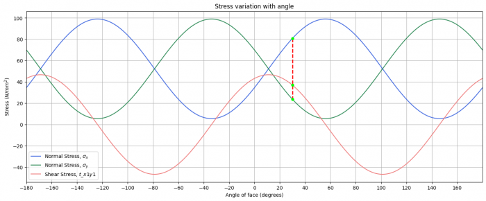
— sig_x1 = 80.8 N/mm^2
— sig_y1 = 23.7 N/mm^2
— tau_x1y1 = 37.0 N/mm^2
(ii) Principal angles
— The principal angles are -33.8 and 56.2 degrees
(iii) Principal stresses
— The principal stresses are 5.5 N/mm^2 occurs on a plane orientatated at -33.8 degrees
— The principal stresses are 99.0 N/mm^2 occurs on a plane orientatated at 56.2 degrees
— sig_1 is 99.0 N/mm^2 and theta_p1 is 56 degrees
— sig_2 is 5.5 N/mm^2 and theta_p2 is -34 degrees
(iv) Planes of max +ve/-ve shear stress
— Max +ve shear stress occurs on a plane at 11.2 degrees
— Max -ve shear stress occurs on a plane at 101.2 degrees
(v) Maximum shear stress
— The maximum shear stress has a magnitude of 46.7 N/mm^2
— The normal stress on the max shear stress planes is 52.2 N/mm^2
(vi) Plotting
F. Cost constraints and optimization
from scipy.optimize import minimize
polymer_price = 60000  # IDR/kg
composite_price = 50000  # IDR/kg
min_polymer = 4  # kg
min_composite = 4  # kg
max_polymer = 27  # kg
max_composite = 23  # kg
max_total_cost = 500000  # IDR
def objective(x):
    polymer_amount = x[0]
    composite_amount = x[1]
    total_cost = polymer_price * polymer_amount + composite_price * composite_amount
    return -total_cost  # Negate the cost to maximize
def constraint1(x):
    polymer_amount = x[0]
    composite_amount = x[1]
    return composite_amount - polymer_amount  # polymer_amount < composite_amount
def constraint2(x):
    polymer_amount = x[0]
    composite_amount = x[1]
    return max_total_cost - (polymer_price * polymer_amount + composite_price * composite_amount)
# Initial guess
x0 = [min_polymer, min_composite]
# Define the bounds and constraints
bounds = [(min_polymer, max_polymer), (min_composite, max_composite)]
constraints = [{'type': 'ineq', 'fun': constraint1}, {'type': 'ineq', 'fun': constraint2}]
# Solve the optimization problem
result = minimize(objective, x0, method='SLSQP', bounds=bounds, constraints=constraints)
# Extract the optimal solution
optimal_polymer_amount = result.x[0]
optimal_composite_amount = result.x[1]
optimal_total_cost = -result.fun
# Print the results
print("Optimal Polymer Amount:", optimal_polymer_amount, "kg")
print("Optimal Composite Amount:", optimal_composite_amount, "kg")
print("Optimal Total Cost:", optimal_total_cost, "IDR")
Optimal Polymer Amount: 4.495855679670058 kg
Optimal Composite Amount: 4.504123774895561 kg
Optimal Total Cost: 494957.5295249815 IDR
G. References
- Neto, E. S. B., Chludzinski, M., Roese, P. B., Fonseca, J., Amico, S. C., & Ferreira, C. R. (2011). Experimental and numerical analysis of a LLDPE/HDPE liner for a composite pressure vessel. Polymer Testing, 30(6), 693–700. https://doi.org/10.1016/j.polymertesting.2011.04.016
- Roh, H. S., Hua, T. Q., & Ahluwalia, R. K. (2013). Optimization of carbon fiber usage in Type 4 hydrogen storage tanks for fuel cell automobiles. International Journal of Hydrogen Energy, 38(29), 12795–12802. https://doi.org/10.1016/j.ijhydene.2013.07.016
- SAE TIR J2579Technical information report for fuel systems in fuel cell and other hydrogen vehicles. USA: Society of Automotive Engineers; 2008.
Final Presentation
"My Conscious Efforts in Numerical Method Learning and Its Application in Hydrogen Storage Design"


